5 Usage (R API)

The following examples illustrate the functionality of {biodosetools}’s R API to perform dose-effect fitting and dose estimation for the dicentric and translocation assays. The equivalent examples using the {shiny} user interface can be found in Chapter 4.

The full {biodosetools} R API reference detailing the available functions and parameters can be found on the project’s website at https://biodosetools-team.github.io/biodosetools/reference/.

5.1 Dicentrics dose-effect fitting

5.1.1 Input count data

The first step is to input the count data. This step is accomplished in R by calling the calculate_aberr_table() function. This will calculate the total number of cells (\(N\)), total number of aberrations (\(X\)), as well as mean (\(\bar{y}\)), variance (\(\sigma^{2}\)), dispersion index (\(\sigma^{2}/\bar{y}\)), and \(u\)-value.

count_data <- system.file("extdata", "count-data-barquinero-1995.csv",
  package = "biodosetools"
) |>
  utils::read.csv() |>
  calculate_aberr_table(type = "count")

count_data

## # A tibble: 11 × 13
##        D     N     X    C0    C1    C2    C3    C4    C5    mean     var    DI
##    <dbl> <int> <dbl> <int> <int> <int> <int> <int> <int>   <dbl>   <dbl> <dbl>
##  1  0     5000     8  4992     8     0     0     0     0 0.0016  0.00160 0.999
##  2  0.1   5002    14  4988    14     0     0     0     0 0.00280 0.00279 0.997
##  3  0.25  2008    22  1987    20     1     0     0     0 0.0110  0.0118  1.08 
##  4  0.5   2002    55  1947    55     0     0     0     0 0.0275  0.0267  0.973
##  5  0.75  1832   100  1736    92     4     0     0     0 0.0546  0.0560  1.03 
##  6  1     1168   109  1064    99     5     0     0     0 0.0933  0.0933  0.999
##  7  1.5    562   100   474    76    12     0     0     0 0.178   0.189   1.06 
##  8  2      333   103   251    63    17     2     0     0 0.309   0.353   1.14 
##  9  3      193   108   104    72    15     2     0     0 0.560   0.466   0.834
## 10  4      103   103    35    41    21     4     2     0 1       0.882   0.882
## 11  5       59   107    11    19    11     9     6     3 1.81    2.09    1.15 
## # … with 1 more variable: u <dbl>

5.1.2 Perform fitting

To perform the fitting in R we call the fit() function, whilst selecting the appropriate aberr_module ("dicentrics" in this example), model_formula ("lin-quad" or "lin" for LQ or L models, respectively), and model_family ("automatic", "poisson", or "quasipoisson") parameters:

fit_results <- fit(
  count_data = count_data,
  model_formula = "lin-quad",
  model_family = "automatic",
  aberr_module = "dicentrics"
)

The fit_results object is a list that contains all necessary information about the count data as well as options selected when performing the fitting. This is a vital step to ensure traceability and reproducibility. Below we can see its elements:

names(fit_results)

##  [1] "fit_raw_data"         "fit_formula_raw"      "fit_formula_tex"     
##  [4] "fit_coeffs"           "fit_cor_mat"          "fit_var_cov_mat"     
##  [7] "fit_dispersion"       "fit_model_statistics" "fit_algorithm"       
## [10] "fit_model_summary"

In particular, we can see how fit_coeffs matches the results obtained in the UI (Figure 4.4):

fit_results$fit_coeffs

##                estimate    std.error statistic      p.value
## coeff_C     0.001280319 0.0004714055  2.715961 6.608367e-03
## coeff_alpha 0.021038724 0.0051576170  4.079156 4.519949e-05
## coeff_beta  0.063032534 0.0040073856 15.729091 9.557291e-56

To visualise the dose-effect curve, we call the plot_fit_dose_curve() function:

plot_fit_dose_curve(
  fit_results,
  aberr_name = "Dicentrics"
)

Plot of dose-effect curve generated by {biodosetools}. The grey shading indicates the uncertainties associated with the calibration curve.

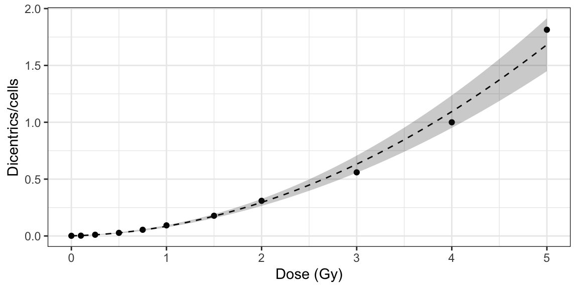
Figure 5.1: Plot of dose-effect curve generated by {biodosetools}. The grey shading indicates the uncertainties associated with the calibration curve.

5.2 Dicentrics dose estimation

5.2.1 Input case data

Next we can choose to either load the case data from a file or to input the data manually. The data is then parsed in R by calling the calculate_aberr_table() function. This will calculate the total number of cells (\(N\)), total number of aberrations (\(X\)), as well as mean (\(\bar{y}\)), standard error (\(\sigma\)), dispersion index (\(\sigma^{2}/\bar{y}\)), and \(u\)-value.

case_data <- system.file("extdata", "cases-data-partial.csv",
  package = "biodosetools"
) |>
  utils::read.csv(header = TRUE) |>
  calculate_aberr_table(
    type = "case",
    assessment_u = 1,
    aberr_module = "dicentrics"
  )

case_data

## # A tibble: 1 × 12
##       N     X    C0    C1    C2    C3    C4    C5     y  y_err    DI     u
##   <int> <int> <int> <int> <int> <int> <int> <int> <dbl>  <dbl> <dbl> <dbl>
## 1   361   100   302    28    22     8     1     0 0.277 0.0368  1.77  10.4

5.2.2 Perform dose estimation

Finally, to perform the dose estimation in R we can call the adequate estimate_*() functions and parameters depending on the characteristics of the accident. In this example, we will use estimate_whole_body_merkle() and estimate_partial_body_dolphin(). First of all, however, we will need to load the fit coefficients and variance-covariance matrix from the previously calculated fit_results:

fit_coeffs <- fit_results$fit_coeffs
fit_var_cov_mat <- fit_results$fit_var_cov_mat

After that is done, we can simply call estimate_whole_body_merkle() and estimate_partial_body_dolphin():

results_whole_merkle <- estimate_whole_body_merkle(
  case_data,
  fit_coeffs,
  fit_var_cov_mat,
  conf_int_yield = 0.83,
  conf_int_curve = 0.83,
  protracted_g_value = 1,
  aberr_module = "dicentrics"
)

results_partial <- estimate_partial_body_dolphin(
  case_data,
  fit_coeffs,
  fit_var_cov_mat,
  conf_int = 0.95,
  gamma = 1 / 2.7,
  aberr_module = "dicentrics"
)

To visualise the estimated doses, we call the plot_estimated_dose_curve() function:

plot_estimated_dose_curve(
  est_doses = list(
    whole = results_whole_merkle,
    partial = results_partial
  ),
  fit_coeffs,
  fit_var_cov_mat,
  protracted_g_value = 1,
  conf_int_curve = 0.95,
  aberr_name = "Dicentrics"
)

Plot of estimated doses generated by {biodosetools}. The grey shading indicates the uncertainties associated with the calibration curve.

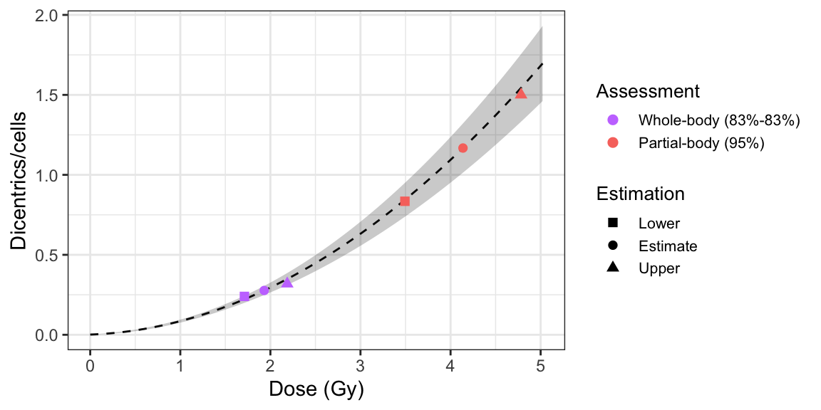
Figure 5.2: Plot of estimated doses generated by {biodosetools}. The grey shading indicates the uncertainties associated with the calibration curve.

5.3 Translocations dose-effect fitting

5.3.1 Calculate genomic conversion factor

To be able to fit the equivalent full genome dose-effect curve, we need to calculate the genomic conversion factor. To calculate the genomic conversion factor in R we call the calculate_genome_factor() function:

genome_factor <- calculate_genome_factor(
  dna_table = dna_content_fractions_morton,
  chromosome = c(1, 4, 11),
  color = rep("Red", 3),
  sex = "female"
)

genome_factor

## [1] 0.3147797

5.3.2 Input count data

Once the genomic conversion factor has been calculated, we can input the count data. This step is accomplished in R by calling the calculate_aberr_table() function. This will calculate the total number of cells (\(N\)), total number of aberrations (\(X\)), as well as mean (\(\bar{y}\)), variance (\(\sigma^{2}\)), dispersion index (\(\sigma^{2}/\bar{y}\)), and \(u\)-value.

count_data <- system.file("extdata", "count-data-rodriguez-2004.csv", package = "biodosetools") |>
  utils::read.csv() |>
  calculate_aberr_table(type = "count") |>
  dplyr::mutate(N = N * genome_factor)

count_data

## # A tibble: 11 × 13
##        D     N     X    C0    C1    C2    C3    C4    C5    mean     var    DI
##    <dbl> <dbl> <dbl> <int> <int> <int> <int> <int> <int>   <dbl>   <dbl> <dbl>
##  1  0    1371.     6  4350     6     0     0     0     0 0.00138 0.00138 0.999
##  2  0.1  1046.    15  3309    15     0     0     0     0 0.00451 0.00449 0.996
##  3  0.25  966.    18  3051    18     0     0     0     0 0.00587 0.00583 0.994
##  4  0.5   967.    33  3039    33     0     0     0     0 0.0107  0.0106  0.990
##  5  0.75  664.    40  2072    38     1     0     0     0 0.0189  0.0195  1.03 
##  6  1     669.    50  2075    48     1     0     0     0 0.0235  0.0239  1.02 
##  7  1.5   328.    56   990    50     3     0     0     0 0.0537  0.0566  1.05 
##  8  2     226.    71   650    65     3     0     0     0 0.0989  0.0976  0.987
##  9  3     246.   157   649   108    23     1     0     0 0.201   0.227   1.13 
## 10  4     125.   147   265   117    15     0     0     0 0.370   0.310   0.836
## 11  5     124.   180   246   122    23     4     0     0 0.456   0.426   0.936
## # … with 1 more variable: u <dbl>

5.3.3 Perform fitting

To perform the fitting in R we call the fit() function, whilst selecting the appropriate aberr_module ("translocations" in this example), model_formula ("lin-quad" or "lin" for LQ or L models, respectively), and model_family ("automatic", "poisson", or "quasipoisson") parameters:

fit_results <- fit(
  count_data = count_data,
  model_formula = "lin-quad",
  model_family = "automatic",
  fit_link = "identity",
  aberr_module = "translocations"
)

names(fit_results)

##  [1] "fit_raw_data"         "fit_formula_raw"      "fit_formula_tex"     
##  [4] "fit_coeffs"           "fit_cor_mat"          "fit_var_cov_mat"     
##  [7] "fit_dispersion"       "fit_model_statistics" "fit_algorithm"       
## [10] "fit_model_summary"

In particular, we can see how fit_coeffs matches the results obtained in the UI (Figure 4.13):

fit_results$fit_coeffs

##                estimate   std.error statistic      p.value
## coeff_C     0.006560406 0.002052834  3.195780 2.538519e-02
## coeff_alpha 0.027197296 0.009922177  2.741061 5.081502e-02
## coeff_beta  0.057982322 0.004630926 12.520675 3.100113e-06

To visualise the dose-effect curve, we call the plot_fit_dose_curve() function:

plot_fit_dose_curve(
  fit_results,
  aberr_name = "Translocations"
)

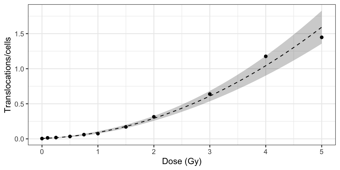
Figure 5.3: Plot of dose-effect curve generated by {biodosetools}. The grey shading indicates the uncertainties associated with the calibration curve.

5.4 Translocations dose estimation

5.4.1 Calculate genomic conversion factor

To be able to fit the equivalent full genome case data, we need to calculate the genomic conversion factor.

To do this, in the “Stain color options” box we select the sex of the individual, and the list of chromosomes and stains used for the translocation assay. Clicking on “Generate table” will show a table in the “Chromosome data” box in which we select the chromosome-stain pairs. Clicking on the “Calculate fraction” will calculate the genomic conversion factor.

To calculate the genomic conversion factor in R we call the calculate_genome_factor() function:

genome_factor <- calculate_genome_factor(
  dna_table = dna_content_fractions_morton,
  chromosome = c(1, 2, 3, 4, 5, 6),
  color = c("Red", "Red", "Green", "Red", "Green", "Green"),
  sex = "male"
)

genome_factor

## [1] 0.5847343

5.4.2 Input case data

Next we can choose to either load the case data from a file or to input the data manually. The data is then parsed in R by calling the calculate_aberr_table() function. If needed, the user can select to use confounders (either using Sigurdson’s method, or by inputting the translocation frequency per cell). Once the table is generated and filled, the “Calculate parameters” button will calculate the total number of cells (\(N\)), total number of aberrations (\(X\)), as well as mean (\(\bar{F}_{p}\)), standard error (\(\sigma_{p}\)), dispersion index (\(\sigma^{2}/\bar{y}\)), \(u\)-value, expected translocation rate (\(X_{c}\)), full genome mean (\(\bar{F}_{g}\)), and full genome error (\(\sigma_{g}\)).

case_data <- data.frame(
  C0 = 288, C1 = 52, C2 = 9, C3 = 1
) |>
  calculate_aberr_table(
    type = "case",
    assessment_u = 1,
    aberr_module = "translocations"
  ) |>
  dplyr::mutate(
    Xc = calculate_trans_rate_sigurdson(
      cells = N,
      genome_factor = genome_factor,
      age_value = 30,
      smoker_bool = TRUE
    ),
    Fg = (X - Xc) / (N * genome_factor),
    Fg_err = Fp_err / sqrt(genome_factor)
  )

case_data

## # A tibble: 1 × 13
##       N     X    C0    C1    C2    C3    Fp Fp_err    DI     u    Xc    Fg
##   <int> <int> <int> <int> <int> <int> <dbl>  <dbl> <dbl> <dbl> <dbl> <dbl>
## 1   350    73   288    52     9     1 0.209 0.0259  1.12  1.64  1.02 0.352
## # … with 1 more variable: Fg_err <dbl>

5.4.3 Perform dose estimation

Finally, to perform the dose estimation in R we can call the adequate estimate_*() functions and parameters depending on the characteristics of the accident. In this example, we will use estimate_whole_body_delta(). First of all, however, we will need to load the fit coefficients and variance-covariance matrix from the previously calculated fit_results:

fit_coeffs <- fit_results$fit_coeffs
fit_var_cov_mat <- fit_results$fit_var_cov_mat

Since we have a protracted exposure, we need to calculate the value of \(G(x)\):

protracted_g_value <- protracted_g_function(
  time = 0.5,
  time_0 = 2
)

protracted_g_value

## [1] 0.9216251

After that is done, we can simply call estimate_whole_body_delta():

results_whole_delta <- estimate_whole_body_delta(
  case_data,
  fit_coeffs,
  fit_var_cov_mat,
  conf_int = 0.95,
  protracted_g_value,
  aberr_module = "translocations"
)

To visualise the estimated doses, we call the plot_estimated_dose_curve() function:

plot_estimated_dose_curve(
  est_doses = list(whole = results_whole_delta),
  fit_coeffs,
  fit_var_cov_mat,
  protracted_g_value,
  conf_int_curve = 0.95,
  aberr_name = "Translocations"
)

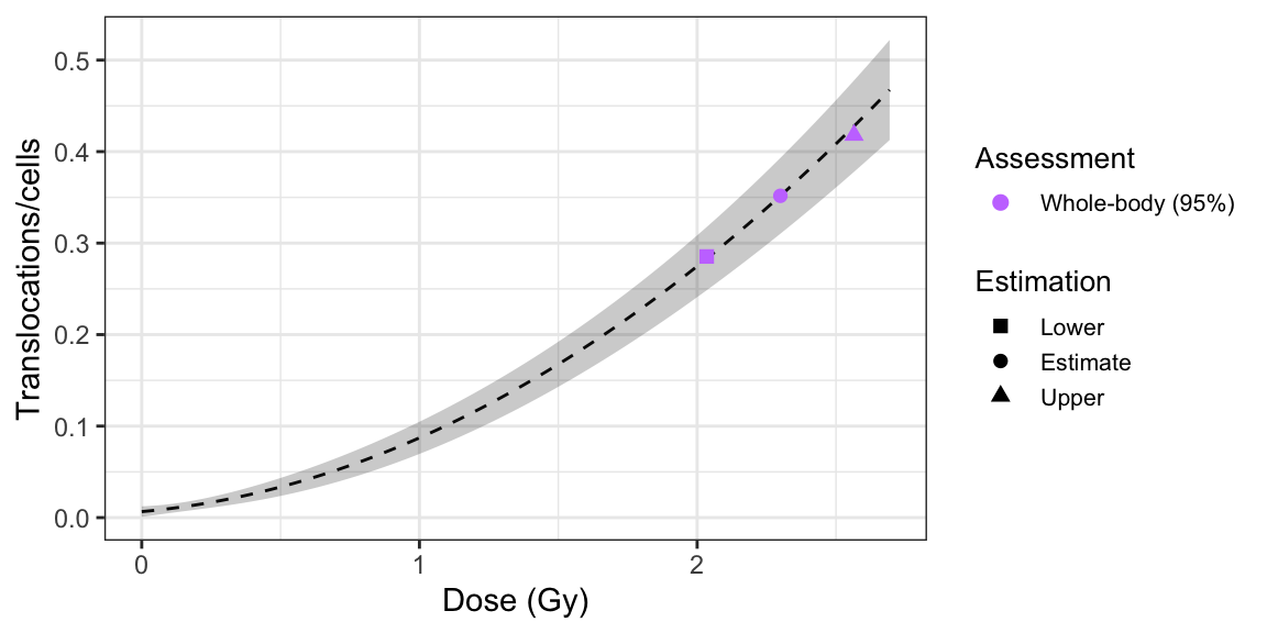
Figure 5.4: Plot of estimated doses generated by {biodosetools}. The grey shading indicates the uncertainties associated with the calibration curve.

4 Usage (web UI)

6 Technical matters