4 Usage (web UI)

The following examples illustrate the functionality of {biodosetools}’s {shiny} user interface to perform dose-effect fitting and dose estimation for the dicentric and translocation assays. The equivalent examples using the R API can be found in Chapter 5.

4.1 Dicentrics dose-effect fitting

4.1.1 Input count data

The first step is to input the count data. On the {shiny} app, we can select to either load the count data from a file (supported formats are .csv, .dat, and .txt) or to input the data manually (Figure 4.1). Once the table is generated and filled (Figure 4.2), the “Calculate parameters” button will calculate the total number of cells ($N$), total number of aberrations ($X$), as well as mean ($\bar{y}$), variance ($\sigma^{2}$), dispersion index ($\sigma^{2}/\bar{y}$), and $u$-value.

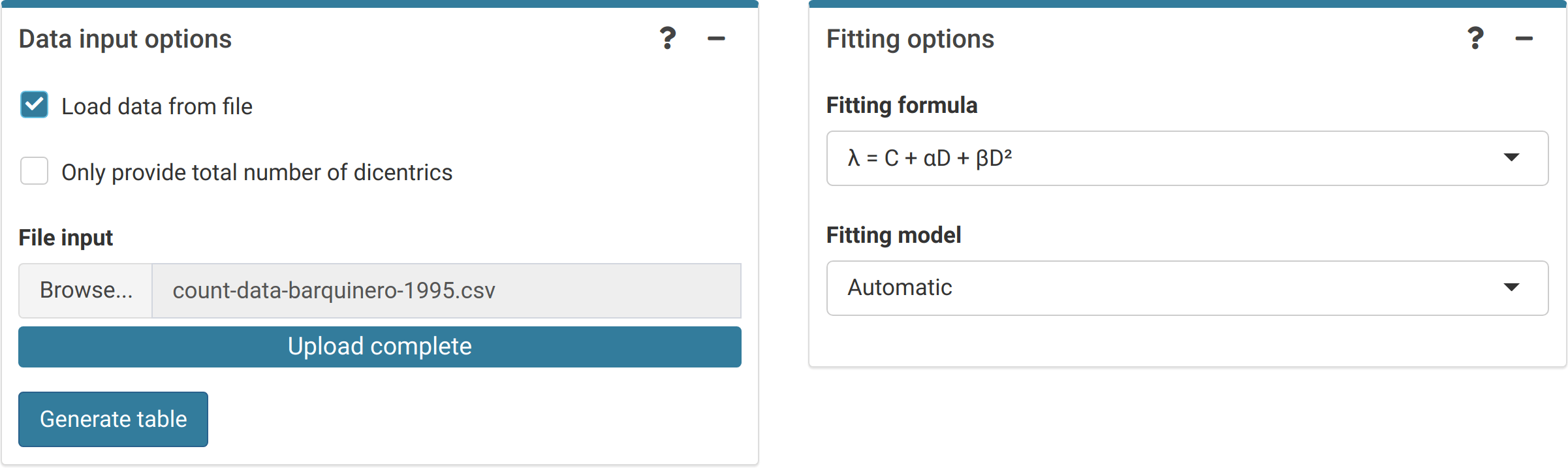
'Data input options' and 'Fitting options' boxes in the dose-effect fitting module. For dicentrics, the 'Automatic' fitting model will select a quasi-Poisson model if there is overdispersion on the fitting, otherwise it will select a Poisson model assuming equidispersion.

Figure 4.1: ‘Data input options’ and ‘Fitting options’ boxes in the dose-effect fitting module. For dicentrics, the ‘Automatic’ fitting model will select a quasi-Poisson model if there is overdispersion on the fitting, otherwise it will select a Poisson model assuming equidispersion.

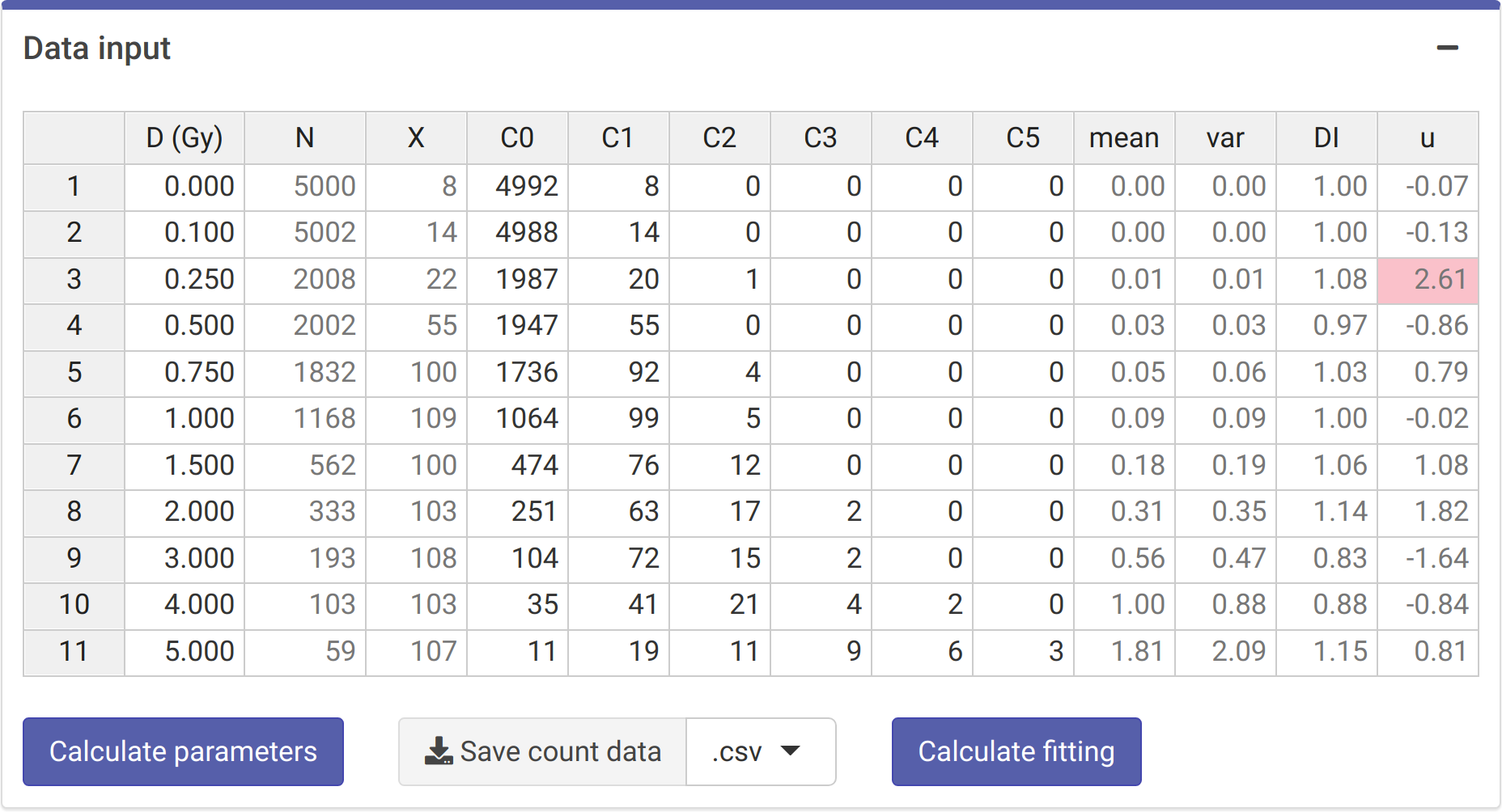
Figure 4.2: `Data input’ box in the dose-effect fitting module.

4.1.2 Irradiation conditions

Because irradiation conditions during calibration may influence future dose estimates (Trompier et al. 2017), and for a better traceability, the user can input the conditions under which the samples used to construct the curve were irradiated. This option is only available in the {shiny} app (Figure 4.3), so that these can be saved into the generated reports.

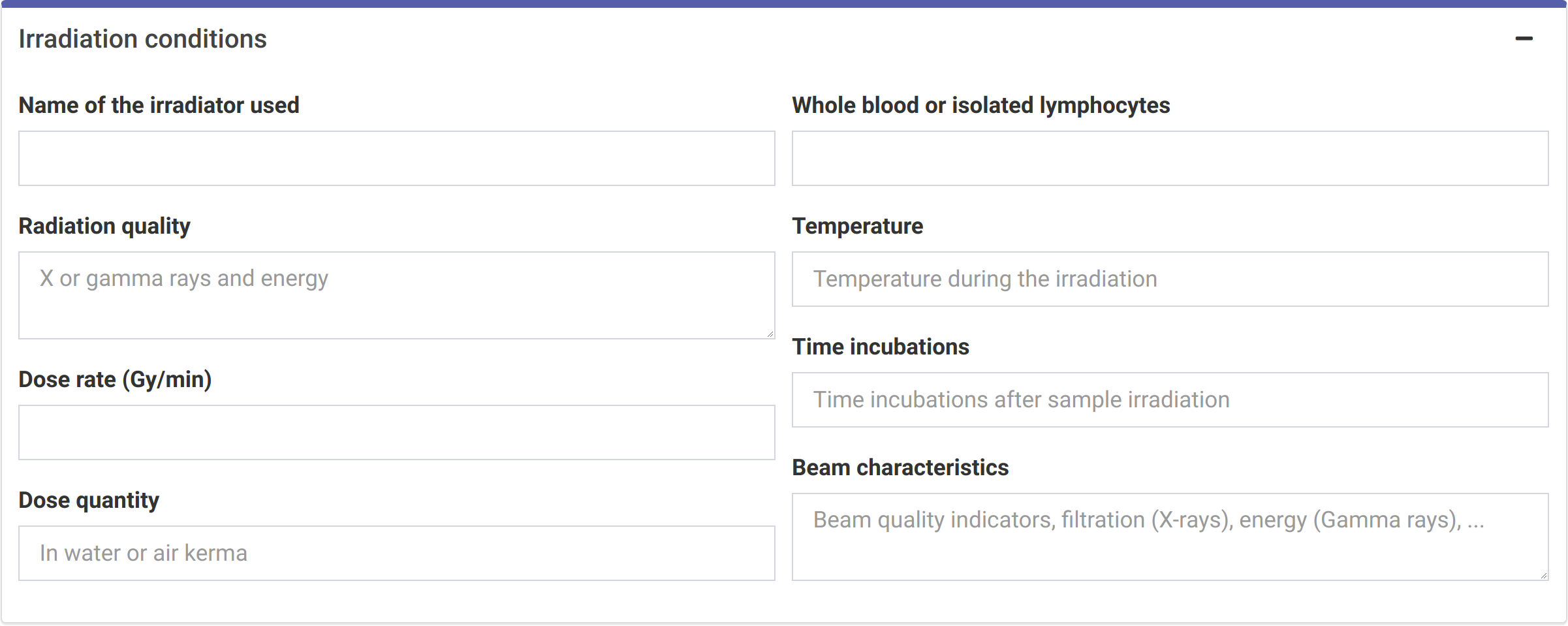
Figure 4.3: ‘Irradiation conditions’ box in the dose-effect fitting module.

4.1.3 Perform fitting

To perform the fitting the user needs to select the appropriate fitting options (Figure 4.1), and then click on the “Calculate fitting” button on the “Data input” box (Figure 4.2). The fitting results and summary statistics are shown in the “Results” tabbed box, and the dose-effect curve is displayed in the “Curve plot” box (Figure 4.4).

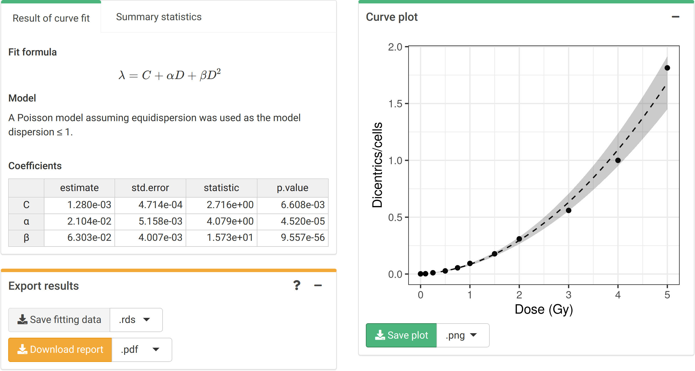
Figure 4.4: ‘Results’ tabbed box, ‘Curve plot’ and ‘Export results’ boxes in the dose-effect fitting module.

The “Export results” box (Figure 4.4) shows two buttons: (a) “Save fitting data”, and (b) “Download report”. The “Save fitting data” will generate an .rds file that contains all information about the count data, irradiation conditions, and options selected when performing the fitting. This file can then be loaded in the dose estimation module to load the dose-effect curve coefficients. Similarly, the “Download report” will generate a .pdf or a .docx report containing all inputs and fitting results.

4.2 Dicentrics dose estimation

4.2.1 Load pre-calculated curve

The first step is to either load the pre-calculated curve in .rds format obtained in the dose-effect fitting module (Figure 4.5) or input the curve coefficients manually (Figure 4.6) in case the user wants to use a pre-existing curve calculated outside of Biodose Tools. Clicking on “Preview data” will load the curve into the app and display it on the “Results” tabbed box.

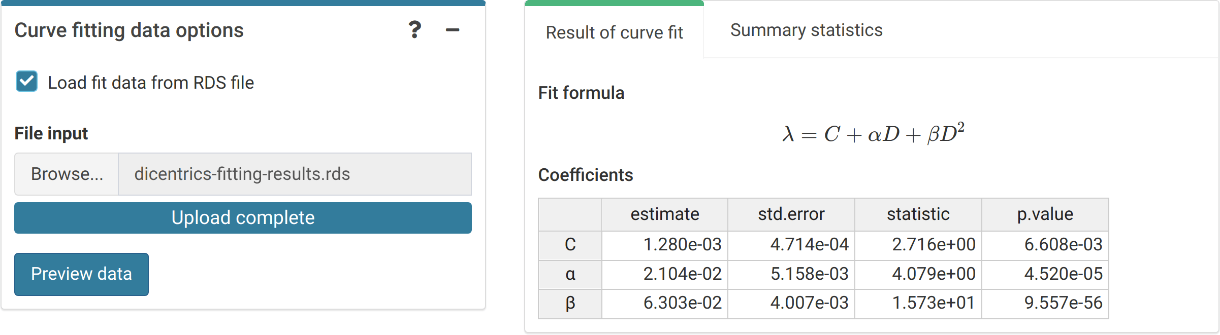
$'Curve fitting data options' box and 'Results' tabbed box in the dose estimation module when loading curve from an \texttt{.rds} file.$

Figure 4.5: ‘Curve fitting data options’ box and ‘Results’ tabbed box in the dose estimation module when loading curve from an file.

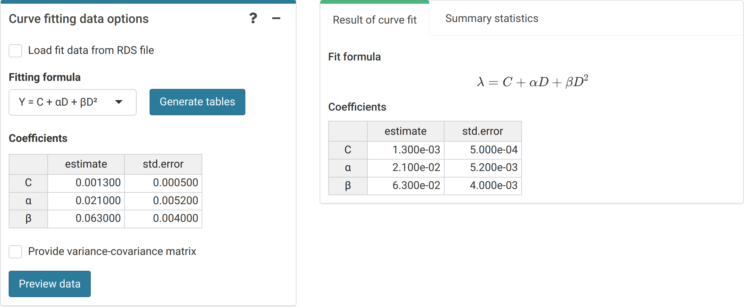
$'Curve fitting data options' box and 'Results' tabbed box in the dose estimation module when inputting curve coefficients manually. Note that if no variance-covariance matrix is provided, only the variances calculated from the coefficients' standard errors will be used in \@ref(eq:merkle-dose-estimation-error), \@ref(eq:delta-method-dose-var), and \@ref(eq:dolphin-method-fraction-F-var).$

Figure 4.6: ‘Curve fitting data options’ box and ‘Results’ tabbed box in the dose estimation module when inputting curve coefficients manually. Note that if no variance-covariance matrix is provided, only the variances calculated from the coefficients’ standard errors will be used in (9.1), (9.4), and (9.14).

4.2.2 Input case data

Next we can choose to either load the case data from a file (supported formats are .csv, .dat, and .txt) or to input the data manually (Figure 4.7). Once the table is generated and filled, the “Calculate parameters” button will calculate the total number of cells ($N$), total number of aberrations ($X$), as well as mean ($\bar{y}$), standard error ($\sigma$), dispersion index ($\sigma^{2}/\bar{y}$), and $u$-value.

The {shiny} app also includes the option to include the information about the incident that is being evaluated. This information may be relevant to explain the results obtained and is included in the generated reports.

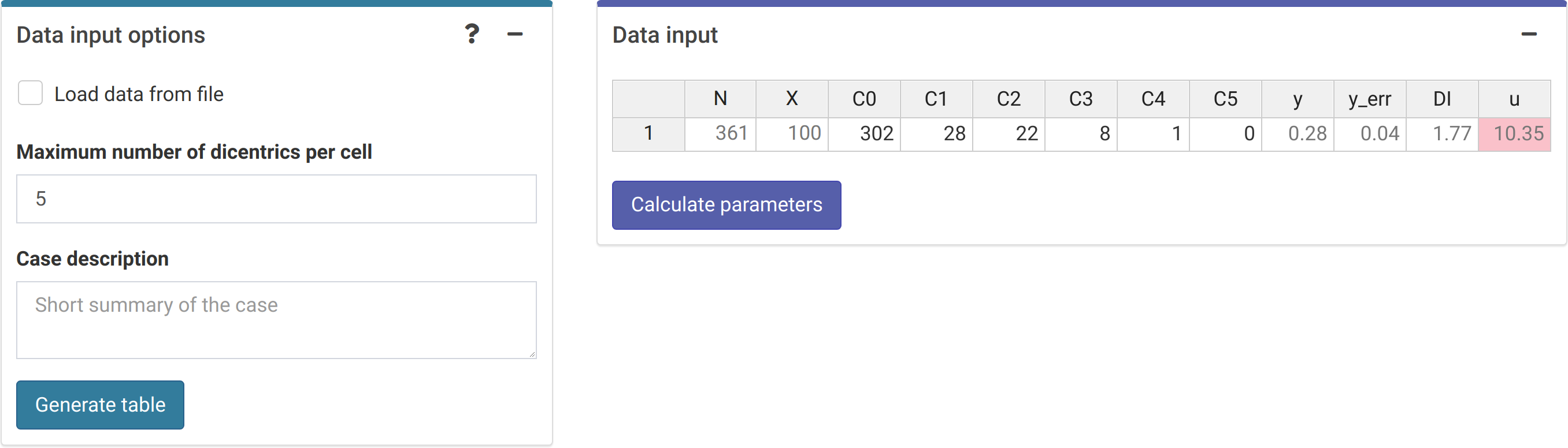
Figure 4.7: ‘Data input options’ and ‘Data input’ boxes in the dose estimation module.

4.2.3 Perform dose estimation

The final step is to select the dose estimation options depending on the characteristics of the accident. In the “Dose estimation options” box (Figure 4.8) we can select type of exposure (acute, protracted, and highly protracted), type of assessment (whole-body, partial-body, or heterogeneous), and error methods for each type of assessment.

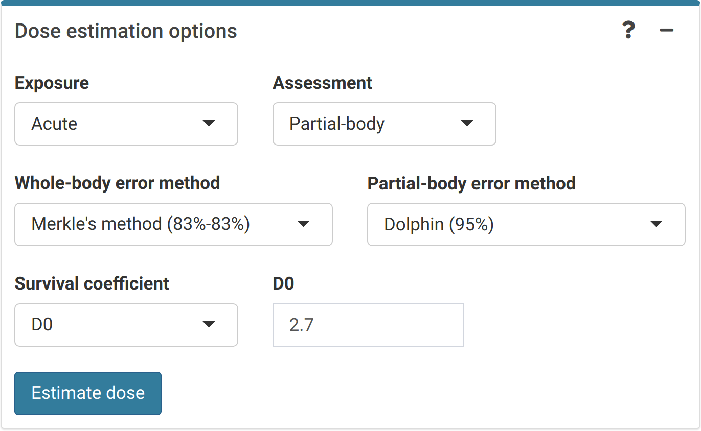
Figure 4.8: ‘Dose estimation options’ box in the dose estimation module.

The dose estimation results are shown in Figure 4.9. Once the estimation is done the app also incorporates the possibility to describe the results obtained in the “Save results” box. All information, the calibration curve used, the data of the case, the different estimated doses, as well as the description of the case and the interpretation of the results can be saved generating a .pdf or a .docx report via the “Download report” button.

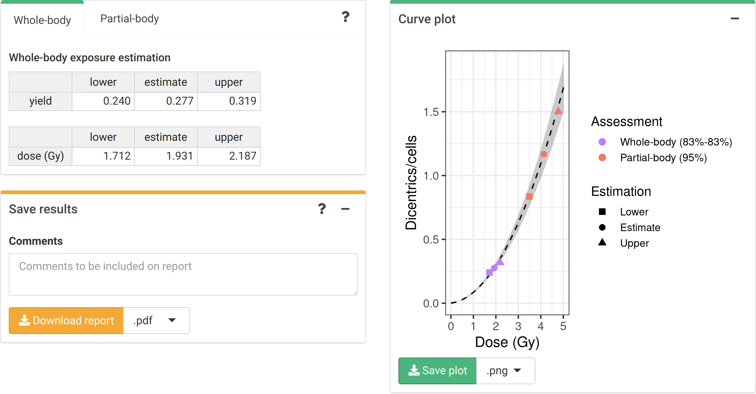
Figure 4.9: ‘Results’ tabbed box, ‘Curve plot’ and ‘Save results’ boxes in the dose estimation module.

It is important to note that {biodosetools} can be used not only to estimate the doses, but also to draft a report of the accident being evaluated with full traceability. This can be further adapted and customised to each laboratory’s internal needs thanks to the open-source nature of the project.

4.3 Translocations dose-effect fitting

4.3.1 Calculate genomic conversion factor

To be able to fit the equivalent full genome dose-effect curve, we need to calculate the genomic conversion factor.

To do this, in the “Stain color options” (Figure 4.10) box we select the sex of the individual, and the list of chromosomes and stains used for the translocation assay. Clicking on “Generate table” will show a table in the “Chromosome data” box in which we select the chromosome-stain pairs. Clicking on the “Calculate fraction” will calculate the genomic conversion factor.

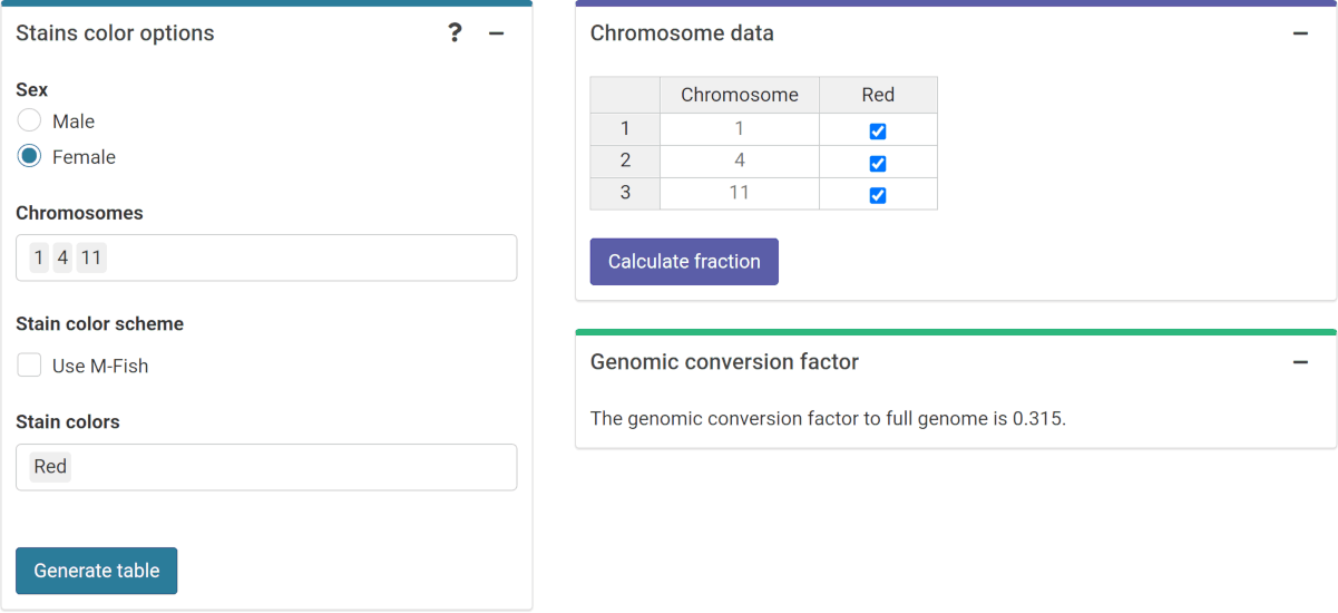
Figure 4.10: ‘Stains color options’, ‘Chromosome data’ and ‘Genomic conversion factor’ boxes in the dose-effect fitting module.

4.3.2 Input count data

Once the genomic conversion factor has been calculated, we can input the count data. On the {shiny} app, we can select to either load the count data from a file (supported formats are .csv, .dat, and .txt) or to input the data manually (Figure 4.11). Once the table is generated and filled @ref(Figure (fig:sc-trans-fit-03)), the “Calculate parameters” button will calculate the total number of cells ($N$), total number of aberrations ($X$), as well as mean ($\bar{y}$), variance ($\sigma^{2}$), dispersion index ($\sigma^{2}/\bar{y}$), and $u$-value.

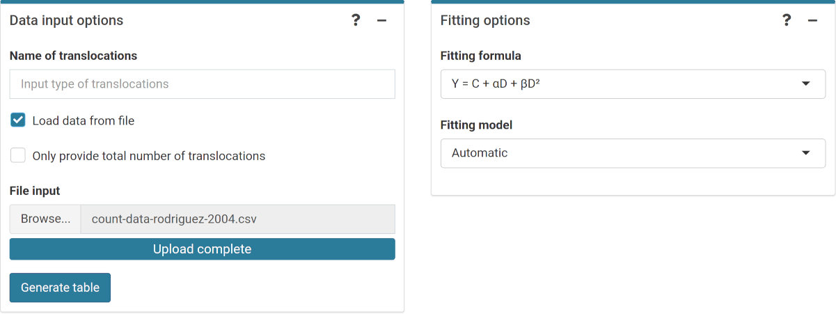
Figure 4.11: ‘Data input options’ and ‘Fitting options’ boxes in the dose-effect fitting module.

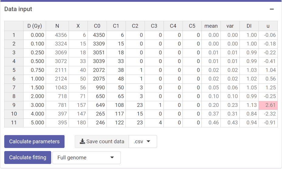
Figure 4.12: ‘Data input’ box in the dose-effect fitting module.

4.3.3 Perform fitting

To perform the fitting the user needs to select the appropriate fitting options (Figure 4.11) to click the “Calculate fitting” button on the “Data input” box (Figure 4.12). The fit can be done either using the full genome translocations, or those measured by FISH. This will not impact any future dose estimation, as the results internally use the full genome translocations. The fitting results and summary statistics are shown in the “Results” tabbed box, and the dose-effect curve is displayed in the “Curve plot” box (Figure 4.13).

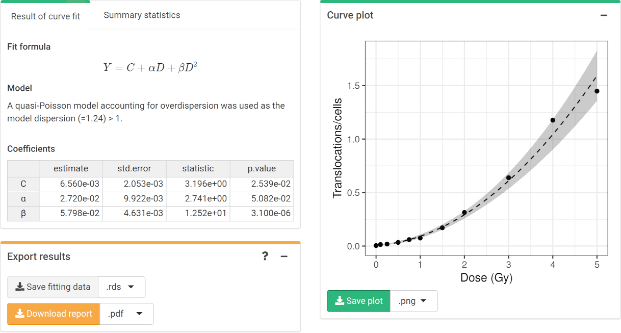
Figure 4.13: ‘Results’ tabbed box, ‘Curve plot’ and ‘Export results’ boxes in the dose-effect fitting module.

The “Export results” box (Figure 4.13) shows two buttons: (a) “Save fitting data”, and (b) “Download report”. The “Save fitting data” will generate an .rds file that contains all information about the count data, irradiation conditions, and options selected when performing the fitting. This file can be then loaded in the dose estimation module to load the dose-effect curve coefficients. Similarly, the “Download report” will generate a .pdf or a .docx report containing all inputs and fitting results.

4.4 Translocations dose estimation

4.4.1 Load pre-calculated curve

The first step is to either load the pre-calculated curve in .rds format obtained in the dose-effect fitting module (Figure 4.14) or input the curve coefficients manually (Figure 4.15) in case the user wants to use a pre-existing curve calculated outside of Biodose Tools. Clicking on “Preview data” will load the curve into the app and display it on the “Results” tabbed box.

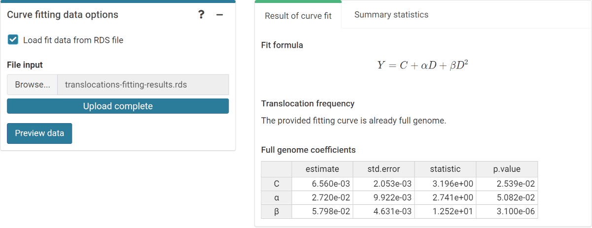
Figure 4.14: ‘Curve fitting data options’ box and ‘Results’ tabbed box in the dose estimation module when loading curve from an .rds file.

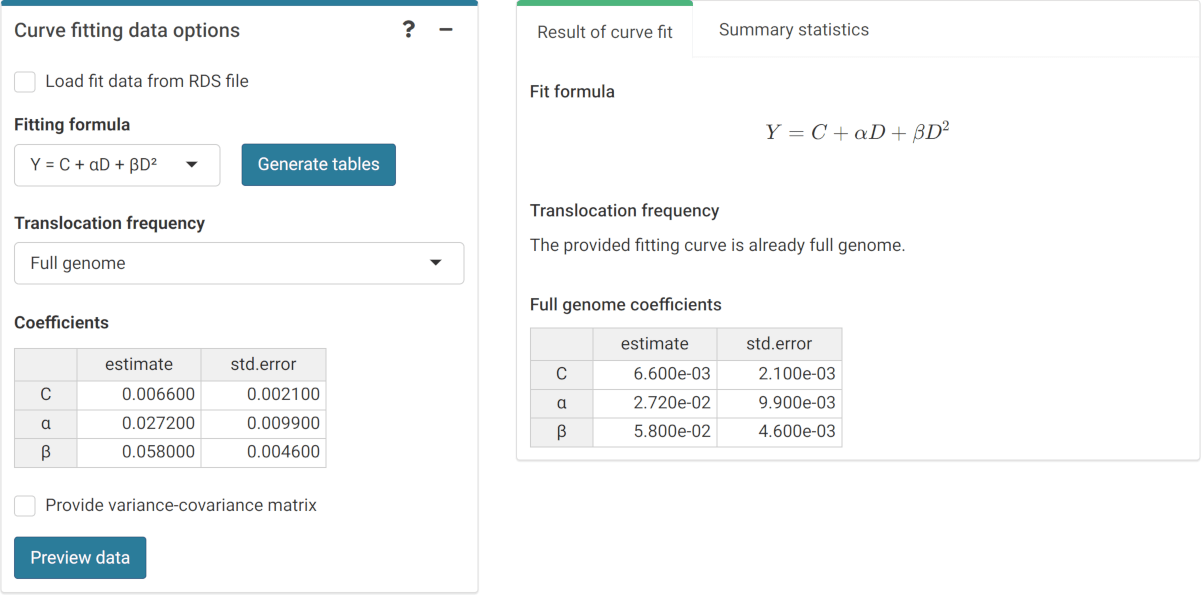
Figure 4.15: ‘Curve fitting data options’ box and ‘Results’ tabbed box in the dose estimation module when inputting curve coefficients manually. Note that if no variance-covariance matrix is provided, only the variances calculated from the coefficients’ standard errors will be used in (9.1), (9.4), and (9.14).

4.4.2 Calculate genomic conversion factor

To be able to fit the equivalent full genome case data, we need to calculate the genomic conversion factor.

To do this, in the “Stain color options” box (Figure 4.16) we select the sex of the individual, and the list of chromosomes and stains used for the translocation assay. Clicking on “Generate table” will show a table in the “Chromosome data” box in which we select the chromosome-stain pairs. Clicking on the “Calculate fraction” will calculate the genomic conversion factor.

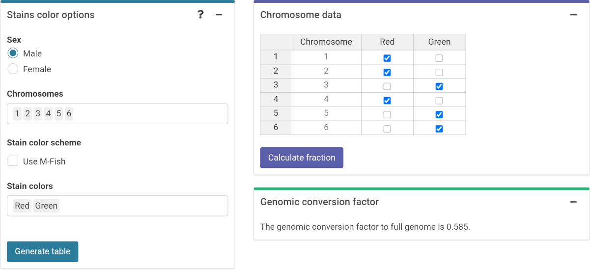
Figure 4.16: ‘Stains color options’, ‘Chromosome data’ and ‘Genomic conversion factor’ boxes in the dose estimation module.

4.4.3 Input case data

Next we can choose to either load the case data from a file (supported formats are .csv, .dat, and .txt) or to input the data manually (Figure 4.17). If needed, the user can select to use confounders (either using Sigurdson’s method, or by inputting the translocation frequency per cell). Once the table is generated and filled, the “Calculate parameters” button will calculate the total number of cells ($N$), total number of aberrations ($X$), as well as mean ($\bar{F}_{p}$), standard error ($\sigma_{p}$), dispersion index ($\sigma^{2}/\bar{y}$), $u$-value, expected translocation rate ($X_{c}$), full genome mean ($\bar{F}_{g}$), and full genome error ($\sigma_{g}$).

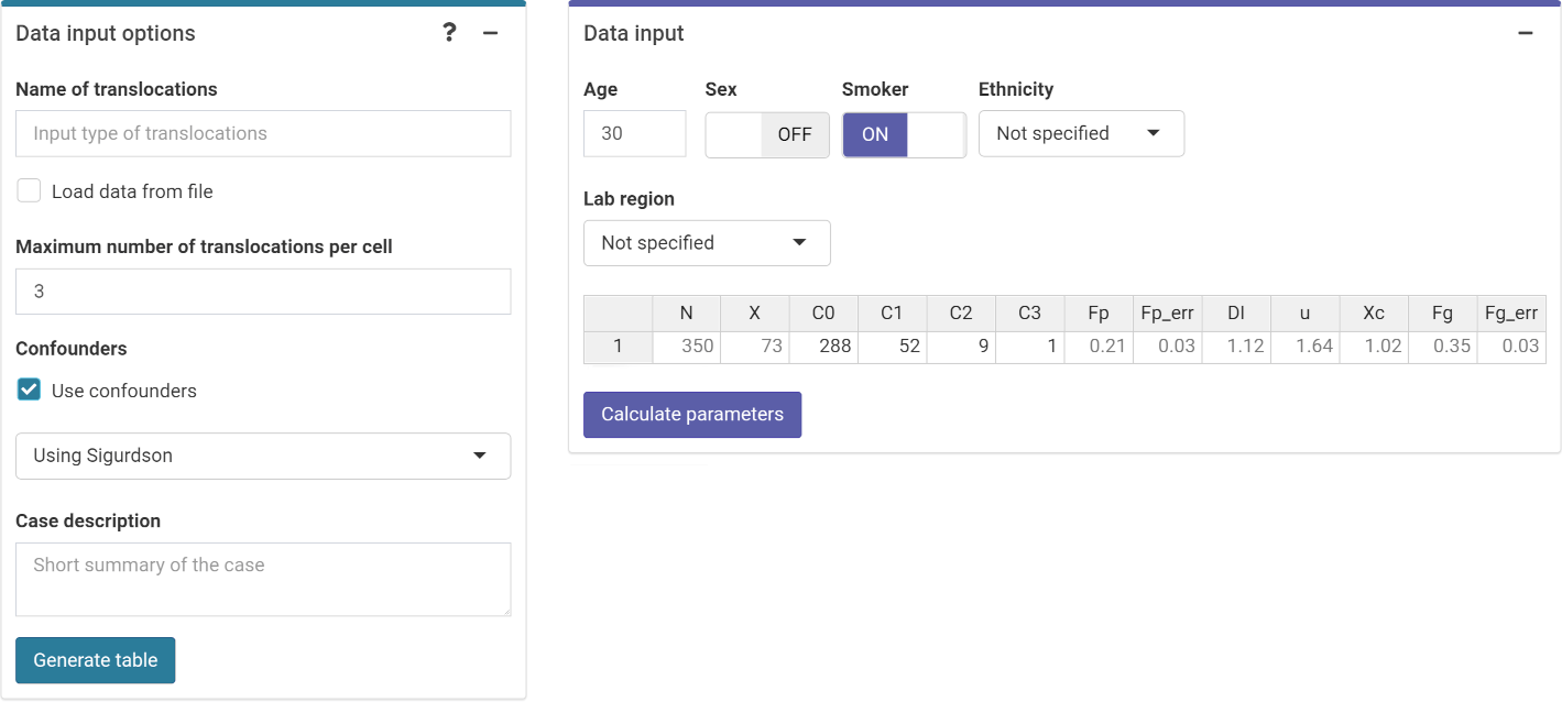
Figure 4.17: ‘Data input options’ and ‘Data input’ boxes in the dose estimation module.

4.4.4 Perform dose estimation

The final step is to select the dose estimation options depending on the characteristics of the accident. In the “Dose estimation options” box (Figure 4.18) we can select type of exposure (acute or protracted), type of assessment (whole-body or partial-body), and error methods for each type of assessment.

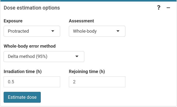
Figure 4.18: ‘Dose estimation options’ box in the dose estimation module.

The dose estimation results are shown in Figure 4.19. Once the estimation is done the app also incorporates the possibility to describe the results obtained in the “Save results” box. All information, the calibration curve used, the data of the case, the different estimated doses, as well as the description of the case and the interpretation of the results can be saved generating a .pdf or a .docx report via the “Download report” button.

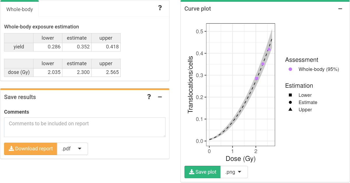
Figure 4.19: ‘Results’ tabbed box, ‘Curve plot’ and ‘Save results’ boxes in the dose estimation module.

3 Getting Biodose Tools

5 Usage (R API)