6 Technical matters
Biodose Tools has been developed following international guidelines of biological dosimetry .
Despite our best efforts to ensure that {biodosetools} automatically handles mathematical errors behind the scenes, such as using a constraint maximum-likelihood optimisation method (Oliveira et al. 2016) when the fitting using a generalized linear model (GLM) is not possible, or correcting negative dose estimates, if the aberration distributions are not well constructed,the resulting curves may still result in errors (both using the {shiny} app or the R API) when performing dose estimation. As an example, let us consider the following curve, shown in Table 6.1 and Figure 6.1. Although at a glance we can already suspect that there is some kind of issue in the observed counts, due to the low number of evaluated cells, one may still decide to proceed and use it for dose estimations.
| \(D \text{ (Gy)}\) | \(N\) | \(X\) |
|---|---|---|
| 0.000 | 100 | 0 |
| 0.250 | 200 | 1 |
| 0.500 | 161 | 6 |
| 1.000 | 88 | 10 |
| 1.500 | 131 | 28 |
| 2.000 | 74 | 23 |
| 2.500 | 189 | 70 |
| 3.000 | 141 | 61 |
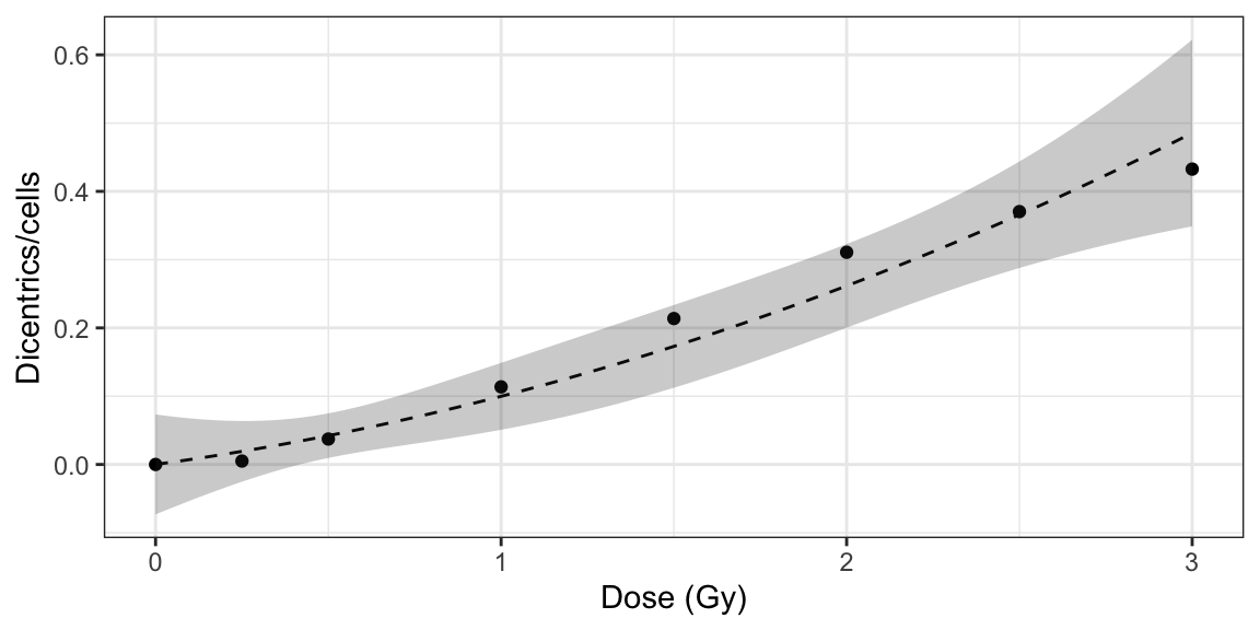
Figure 6.1: Plot of dose-effect curve constructed from the dicentric distribution in Table 6.1.
In Table 6.2 below we can see an example of a case we may want to estimate the dose for. If we try to estimate the dose using Merkle’s method, we encounter an error involving the uniroot() function. The function uniroot() searches for a root (i.e., zero) of the function \(f(x_{1}, \dots, x_{n})\) with respect to its first argument \(x_{1}\) within a specified interval. In our example, this error occurs when projecting the upper 95% confidence limit of the yield \(\lambda_{U}\) into the lower curve (9.1). The reason for this is that the lower 95% confidence band of the dose-effect curve is not a monotonically increasing function, meaning that \(D_{L}\) has multiple possible numerical solutions, as shown in Figure 6.2.
| ID | \(N\) | \(C_{0}\) | \(C_{1}\) | \(C_{2}\) | \(X\) | \(y\) | \(\hat{\sigma}_{y} / \sqrt{N}\) | \(\hat{\sigma}^{2} / \bar{y}\) | \(u\) |
|---|---|---|---|---|---|---|---|---|---|
| Case1 | 148 | 13 | 136 | 11 | 1 | 0.08783784 | 0.02523844 | 1.07326 | 0.6537205 |
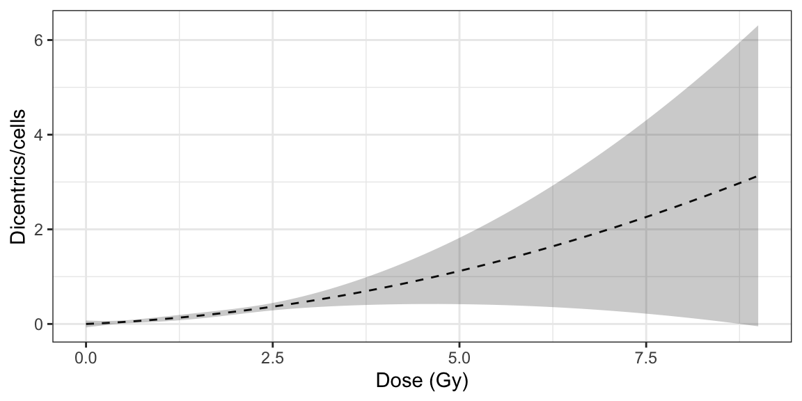
Figure 6.2: Plot of dose-effect curve constructed from the dicentric distribution in Table 6.1 over an extended \(D\) range.
It is worth noting that this projection error is particular to Merkle’s method for whole-body assessment and could certainly be circumvented if one chooses to use the delta method instead. However, for optimal dose estimation we expect both the calibration curve and its confidence intervals to define monotonically increasing functions.