9 Uncertainty on dose estimation

While it is simple to determine a dose from a measured yield of dicentrics, the associated uncertainty can be calculated using a variety of methods. Calculating 95% confidence limits is a common procedure for expressing uncertainty in terms of a confidence interval. A frequentist 95% confidence interval means that with a large number of repeated samples, 95% of such calculated confidence intervals would include the true value of the dose. The problem in estimating confidence limits for dicentrics and translocations after low-LET exposure comes from two sources of uncertainty: the uncertainty from the aberration yield of the person to be examined, and uncertainties associated with the calibration curve. This issue has been discussed in the literature (Merkle 1983; Savage et al. 2000; Szłuińska, Edwards, and Lloyd 2007).

Depending on the type of exposure, methods for whole-body assessment, partial-body assessment, and heterogeneous exposures with two different doses were implemented in the {biodosetools} package, using the following methods. The {biodosetools} package implements the following assessment methods, which are indicated in International Atomic Energy Agency (2001) and International Atomic Energy Agency (2011):

• Whole-body assessment: Merkle’s method (Merkle 1983).
• Whole-body assessment: delta method (International Atomic Energy Agency 2001).
• Partial-body assessment: Dolphin’s method (Dolphin 1969).

In addition {biodosetools} also includes a method to assess heterogeneous exposures using a mixed Poisson model (Pujol et al. 2016). That was used in a recent RENEB/EURADOS field exercise (Endesfelder et al. 2021).

9.1 Whole-body assessment: Merkle’s method

The simplest solution for whole-body assessment was proposed by Merkle (1983), it allows both the Poisson error on the yield and the errors on the calibration curve to be taken into account.

Merkle’s approach, illustrated in Figure 9.1, involves the following steps:

1. Assuming the Poisson (or quasi-Poisson) distribution, calculate the yields corresponding to lower and upper confidence limits on the observed yield \(\lambda\) (\(\lambda_{L}\) and \(\lambda_{U}\)).
2. Calculate the confidence limits of the dose-effect calibration curve according to: \[\begin{align} \begin{aligned} \lambda ={}& C + \alpha D + \beta G(x) D^{2} \\ &\pm R \sqrt{ \begin{aligned} {}& \sigma_{C}^{2} + \sigma_{\alpha}^{2} D^{2} + \sigma_{\beta}^{2} G(x) D^{4} + 2 \sigma_{C, \alpha} D \\ & + 2 \sigma_{C, \beta} G(x) D^{2} + 2 \sigma_{\alpha, \beta} G(x) D^{3} \end{aligned} }, \end{aligned} \tag{9.1} \end{align}\] where \(R^{2}\) is the confidence factor, defined as an upper-confidence limit of a chi-square distribution, \(\chi^{2}(\nu)\), with 2 or 3 degrees of freedom (\(\nu\)).
3. Calculate the dose at which \(\lambda\) crosses the dose-effect calibration curve. This is the estimated dose (\(D\)). For this we can simply take the inverse of the LQ dose-effect calibration curve, as follows: \[\begin{align} D = \frac{-\alpha + \sqrt{\alpha^{2} + 4 \beta G(x) (\lambda - C)}}{2 \beta G(x)}. \tag{9.2} \end{align}\]
4. Calculate the dose at which \(\lambda_{L}\) crosses the upper curve. This is the lower confidence limit of the dose (\(D_{L}\)).
5. Calculate the dose at which \(\lambda_{U}\) crosses the lower curve. This is the upper confidence limit of the dose (\(D_{U}\)).

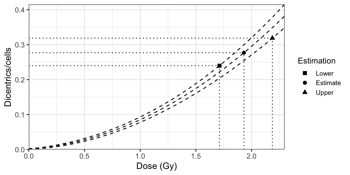
Figure 9.1: A dose-effect calibration curve with its 83% confidence limits, used to estimate dose uncertainties using Merkle’s method.

As suggested by some authors, in order to reduce a possible overestimation of the uncertainty (Schenker and Gentleman 2001; Austin and Hux 2002), it is recommended to use an 83% confidence limit of the regression curve when overlapped with the Poisson 83% confidence limits, as this tends to yield a global 95% confidence interval for the dose estimation.

9.2 Whole-body assessment: delta method

Another approach for whole-body assessment is using the delta method (International Atomic Energy Agency 2001). It also allows both the Poisson error on the yield and the errors on the calibration curve to be taken into account.

The delta method expands a function of a set of random variables \(f(X_{1}, X_{2}, \dots, X_{n})\) about its mean, usually with a first-order Taylor expansion, and then takes the variance. Using the delta method, the variance \(\sigma_{f}^{2}\) of \(f(X_{1}, X_{2}, \dots, X_{n})\) can be expressed as follows (Klein 1953): \[\begin{align} \sigma_{f}^{2} = \sum_{i}^{n} \left(\frac{\partial f}{\partial X_{i}} \right)^{2} \sigma_{X_{i}}^{2} + \sum_{i}^{n} \sum_{j \neq i}^{n} \frac{\partial f}{\partial X_{i}} \frac{\partial f}{\partial X_{j}} \sigma_{X_{i}, X_{j}}. \tag{9.3} \end{align}\]

The approach using the delta method, illustrated in Figure 9.2, involves the following steps:

1. Calculate the dose at which \(\lambda\) crosses the dose-effect calibration curve. This is the estimated dose (\(D\)). For this we can simply take the inverse of the LQ dose-effect calibration curve, as shown in (9.2).
2. By differentiation of the above equation, express the variance on the estimated dose (\(\sigma_{D}^{2}\)) in terms of the variances and co-variances of \(C\), \(\alpha\), \(\beta\), and \(\lambda\). The formal expression is as follows: \[\begin{align} \begin{aligned} \sigma_{D}^{2} ={}& \left(\frac{\partial D}{\partial C} \right)^{2} \sigma_{C}^{2} + \left(\frac{\partial D}{\partial \alpha} \right)^{2} \sigma_{\alpha}^{2} + \left(\frac{\partial D}{\partial \beta} \right)^{2} \sigma_{\beta}^{2} + \left(\frac{\partial D}{\partial \lambda} \right)^{2} \sigma_{\lambda}^{2} \\ & + 2 \frac{\partial D}{\partial C} \frac{\partial D}{\partial \alpha} \sigma_{C, \alpha} + 2 \frac{\partial D}{\partial C} \frac{\partial D}{\partial \beta} \sigma_{C, \beta} + 2 \frac{\partial D}{\partial \alpha} \frac{\partial D}{\partial \beta} \sigma_{\alpha, \beta}. \end{aligned} \tag{9.4} \end{align}\] Note that this derivation assumes that the covariances \(\sigma_{\lambda, C}\), \(\sigma_{\lambda, \alpha}\), and \(\sigma_{\lambda, \beta}\) are all zero. This is appropriate because, in general, the measurements used to calculate the calibration curve and those used to determine the patient’s yield are independent. The variance and co-variances on \(C\), \(\alpha\), and \(\beta\) are derived from the fitted calibration curve, whereas the variance on \(\lambda\) is derived according to (7.6).
3. The lower and upper 95% confidence limits of the dose estimation (\(D_{L}\) and \(D_{U}\)) and the yield (\(\lambda_{L}\) and \(\lambda_{U}\)) are then calculated as follows: \[\begin{align} D_{L, U} = D \pm 1.96 \sigma_{D}, \tag{9.5} \\ \lambda_{L, U} = \lambda \pm 1.96 \sigma_{\lambda}. \tag{9.6} \end{align}\]

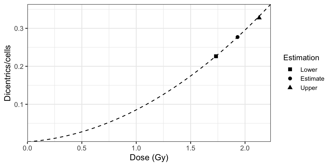
Figure 9.2: A dose-effect calibration curve used to estimate dose uncertainties using delta method.

9.3 Partial-body assessment: Dolphin’s method

This method was first proposed by Dolphin (1969) and is based on a contaminated Poisson method. The chromosomal aberrations distribution of a partial-body irradiation is expected to be overdispersed (\(u > 1.96\)). The observed distribution is considered to be the mixture of (a) a Poisson distribution which represents the irradiated fraction of the body and (b) the remaining unexposed fraction. This method assumes that the background level in the unirradiated part is zero. Undamaged cells will comprise two subpopulations: those from the unexposed fraction and irradiated cells which received no damage.

The distribution of the damage in the irradiated cells can be described by a zero-truncated Poisson distribution with probability function, \[\begin{align} \Pr(Y = k \mid Y > 0) = \frac{P(Y = k)}{1 - P(Y = 0)} = \frac{\lambda^{k}}{(e^{\lambda} - 1)k!} \tag{9.7} \end{align}\]

where \(k \in \{ 1, 2, \dots \}\) and \(Y \sim \operatorname{Pois}(\lambda)\). The distribution of the total number of dicentrics in all the cells can be understood as a zero-inflated Poisson distribution \(Z \sim \operatorname{ZIP}(\lambda, \pi)\) with probability function, \[\begin{align} P(Z = k) = \begin{cases} \pi + (1 - \pi) e^{-\lambda} ,\quad k = 0 \\ (1 - \pi) \dfrac{\lambda^{k} e^{-\lambda}}{k!} ,\quad k \in \{ 1, 2, \dots \} \end{cases} \tag{9.8} \end{align}\] where \(\pi\) is the proportion of extra zeros.

The approach using Dolphin’s method, illustrated in Figure 9.3, involves the following steps:

1. Calculate the yield of dicentrics (\(\lambda\)) in the irradiated fraction by solving the equation, \[\begin{align} \frac{X}{N - C_{0}} = \frac{\lambda}{1 - e^{-\lambda}}, \tag{9.9} \end{align}\] where \(X\) is the total number of dicentrics observed, \(N\) is the total number of cells, and \(C_{0}\) is the number of cells free of dicentrics. The solution \(\lambda\) of this equation is the maximum likelihood estimator (MLE) of the mean yield of dicentrics \(\lambda\) of the zero-truncated Poisson distribution (9.7).
2. Calculate the fraction of cells scored which were irradiated (\(f = 1 - \pi\)) as follows: \[\begin{align} f = \frac{X}{N \lambda}. \tag{9.10} \end{align}\]
3. Calculate the variance on the yield (\(\sigma_{\lambda}^{2}\)), the fraction of cells scored which were irradiated (\(\sigma_{f}^{2}\)), and their covariance (\(\sigma_{f, \lambda}\)) by inverting the observed Fisher information matrix (\(I\)) of the zero-inflated model: \[\begin{align} \begin{pmatrix} \sigma^{2}_{\lambda} & \sigma_{f, \lambda} \\ \sigma_{f, \lambda} & \sigma^{2}_{f} \end{pmatrix} = I^{-1}(\lambda, \pi = 1 - f), \tag{9.11} \end{align}\] where \[\begin{align} I(\lambda, \pi = 1 - f) = \begin{pmatrix} \frac{N f (f - 1)}{f + (1 - f) e^{\lambda}} + \frac{N f}{\lambda} & \frac{N}{f + (1 - f) e^{\lambda}} \\ \frac{N}{f + (1 - f) e^{\lambda}} & \frac{N (e^{\lambda} - 1)}{f (f + (1 - f) e^{\lambda})} \end{pmatrix}. \tag{9.12} \end{align}\]
4. Calculate the dose at which \(\lambda\) crosses the dose-effect calibration curve. This is the estimated dose (\(D\)). For this we can simply take the inverse of the LQ dose-effect calibration curve, as shown in (9.2).
5. Calculate the variance on the estimated dose (\(\sigma_{D}^{2}\)) using the delta method, as shown in (9.4). The variance and co-variances on \(C\), \(\alpha\), and \(\beta\) are derived from the fitted calibration curve, whereas the variance on \(\lambda\) is derived from the inverse of the observed Fisher information matrix (9.11).
6. Calculate the initial fraction of irradiated cells (\(F\)): \[\begin{align} F = \frac{f}{f + (1 - f) e^{-D / D_{0}}}, \tag{9.13} \end{align}\] where \(f\) is the fraction of cells scored which were irradiated, \(D\) is the expression of the estimated dose (9.2), and \(D_{0}\) is the survival coefficient with experimental values between 2.7 and 3.5 (D. C. Lloyd, Purrott, and Dolphin 1973; J. F. Barquinero et al. 1997).
7. Calculate the variance on the initial fraction of irradiated cells (\(\sigma_{F}^{2}\)) using the delta method: \[\begin{align} \begin{aligned} \sigma_{F}^{2} ={}& \left(\frac{\partial F}{\partial f} \right)^{2} \sigma_{f}^{2} + \left(\frac{\partial F}{\partial C} \right)^{2} \sigma_{C}^{2} + \left(\frac{\partial F}{\partial \alpha} \right)^{2} \sigma_{\alpha}^{2} \\ & + \left(\frac{\partial F}{\partial \beta} \right)^{2} \sigma_{\beta}^{2} + \left(\frac{\partial F}{\partial \lambda} \right)^{2} \sigma_{\lambda}^{2} + 2 \frac{\partial F}{\partial f} \frac{\partial F}{\partial \lambda} \sigma_{f, \lambda} \\ & + 2 \frac{\partial F}{\partial C} \frac{\partial F}{\partial \alpha} \sigma_{C, \alpha} + 2 \frac{\partial F}{\partial C} \frac{\partial F}{\partial \beta} \sigma_{C, \beta} + 2 \frac{\partial F}{\partial \alpha} \frac{\partial F}{\partial \beta} \sigma_{\alpha, \beta}. \end{aligned} \tag{9.14} \end{align}\] Note that this derivation assumes that the covariances \(\sigma_{\lambda, C}\), \(\sigma_{\lambda, \alpha}\), \(\sigma_{\lambda, \beta}\), \(\sigma_{f, C}\), \(\sigma_{f, \alpha}\), and \(\sigma_{f, \beta}\) are all zero. The variance and co-variances on \(C\), \(\alpha\), and \(\beta\) are derived from the fitted calibration curve, whereas the variances on \(\lambda\) and \(f\) and covariance \(\sigma_{f, \lambda}\) are derived from the inverse of the observed Fisher information matrix (9.11).
8. The lower and upper 95% confidence limits of the dose estimation (\(D_{L}\) and \(D_{U}\)), the yield (\(\lambda_{L}\) and \(\lambda_{U}\)) are calculated following (9.5) and (9.6), respectively, and the initial fraction of irradiated cells (\(F_{L}\) and \(F_{U}\)) is then calculated as follows: \[\begin{align} F_{L, U} = F \pm 1.96 \sigma_{F}. \tag{9.15} \end{align}\]

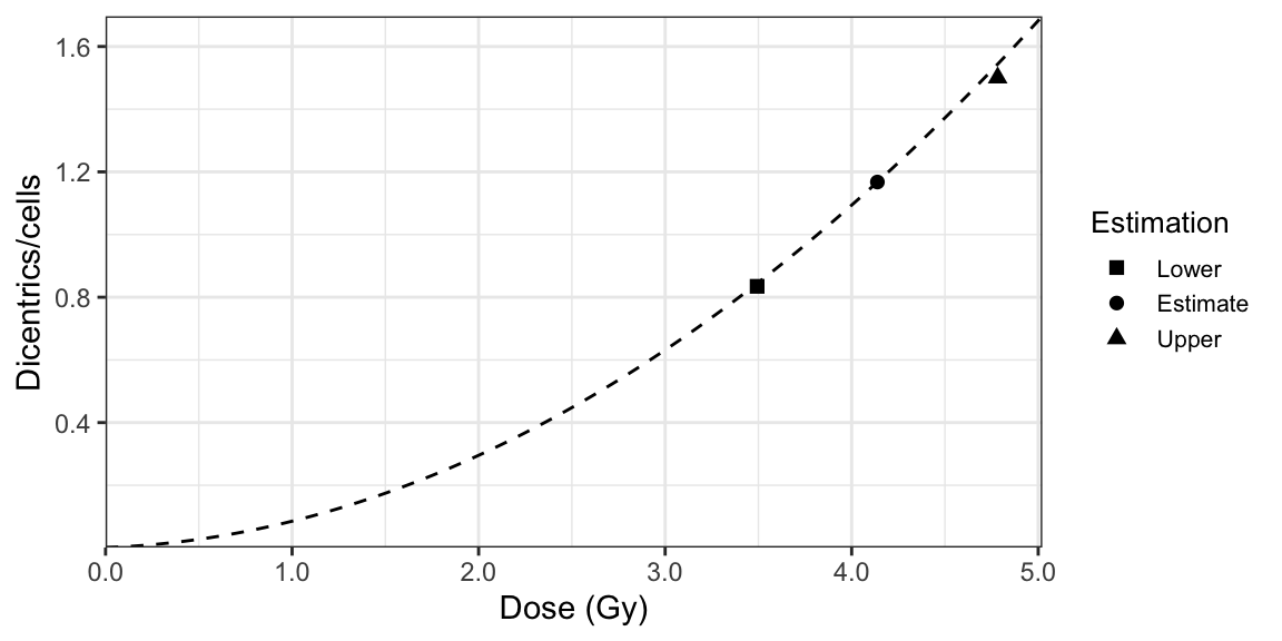
Figure 9.3: A dose-effect calibration curve used to estimate dose uncertainties using Dolphin’s method.

9.4 Heterogeneous assessment: mixed Poisson model

So far, all non-homogeneous exposures have been handled as partial-body exposures with one fraction of the body uniformly irradiated at a certain dose, while the rest of the body is not exposed and hence without chromosome aberrations. This, however, represents a rather idealised situation, since the majority of accidents involve non-uniform exposures, where mixing of almost homogeneously irradiated and nonirradiated blood is extremely unlikely.

To remedy this, a mathematical approach based on a mixed Poisson model (9.16) that can be used in cases of suspected non-homogeneous exposures with two different doses was proposed by Pujol et al. (2016). This model allows to infer two different distributions from an observed dicentric cell distribution.

For a heterogeneous exposure with two radiation doses \(x_{1}\) and \(x_{2}\), the distribution outcome of dicentrics is a mixture of two Poisson distributions (7.3). A random variable \(Y\) distributed as a mixture of two independent Poisson distributions with rates \(\lambda_{1}\) and \(\lambda_{2}\) has the following probability mass function: \[\begin{align} \Pr(Y = k) = \omega \frac{\lambda_{1}^{k} e^{-\lambda_{1}}}{k!} + (1 - \omega) \frac{\lambda_{2}^{k} e^{-\lambda_{2}}}{k!}, \tag{9.16} \end{align}\] where \(\lambda_{1}\) represents the yield of dicentrics for the dose \(x_{1}\), \(\lambda_{2}\) represents the yield for the dose \(x_{2}\) and \(\omega\), a parameter between 0 and 1, represents the population proportion of scored cells that have received a dose \(x_{1}\). Similarly, \(1 - \omega\) can be understood as the population proportion of scored cells that have received a dose \(x_{2}\).

The approach using the mixed Poisson model, illustrated in Figure 9.4, involves the following steps:

1. Calculate the maximum likelihood estimates for the yields (\(\lambda_{1}\) and \(\lambda_{2}\)) and the fraction of scored cells that have received a dose \(D_{1}\) (\(f_{1} = \omega\)) using an optimisation method, such as Limited-memory BFGS-B (Byrd et al. 1995).
2. Calculate the variances on the yields and the fraction of scored cells that have received a dose \(D_{1}\) (\(\sigma_{\lambda_{1}}^{2}\), \(\sigma_{\lambda_{2}}^{2}\), and \(\sigma_{f_{1}}^{2}\)) by inverting the observed Fisher information matrix (\(I\)) resulting from the aforementioned optimisation method: \[\begin{align} \begin{pmatrix} \sigma^{2}_{f_{1}} & \sigma_{f_{1}, \lambda_{1}} & \sigma_{f_{1}, \lambda_{2}} \\ \sigma_{f_{1}, \lambda_{1}} & \sigma^{2}_{\lambda_{1}} & \sigma_{\lambda_{1}, \lambda_{2}} \\ \sigma_{f_{1}, \lambda_{2}} & \sigma_{\lambda_{1}, \lambda_{2}} &\sigma^{2}_{\lambda_{2}} \end{pmatrix} = I^{-1}. \tag{9.17} \end{align}\]
3. Calculate doses at which \(\lambda_{1}\) and \(\lambda_{2}\) cross the dose-effect calibration curve. These are the estimated doses (\(D_{1}\) and \(D_{2}\)). For this we can simply take the inverse of the LQ dose-effect calibration curve, as shown in (9.2).
4. Calculate the variance on the estimated doses (\(\sigma_{D_{i}}^{2}\)) using the delta method, as shown in (9.4). The variances and co-variances on \(C\), \(\alpha\), and \(\beta\) are derived from the fitted calibration curve, whereas the variances on \(\lambda_{i}\) are derived from the inverse of the observed Fisher information matrix (9.17).
5. Calculate the initial fraction of irradiated cells (\(F_{1}\)): \[\begin{align} F_{1} = \frac{f_{1}}{f_{1} + (1 - f_{1}) e^{-\gamma (D_{1} - D_{2})}} ,\quad F_{2} = 1 - F_{1}, \tag{9.18} \end{align}\] where \(f_{1}\) is the fraction of cells scored which were irradiated at the highest dose, \(D_{1}\) and \(D_{2}\) are the estimated doses, \(\gamma = 1 / D_{0}\) is the survival coefficient which is a constant value calculated experimentally from each culture treatment.
6. Calculate the variance on the initial fraction of irradiated cells (\(\sigma_{F_{1}}^{2} = \sigma_{F_{2}}^{2}\)) using the delta method: \[\begin{align} \begin{aligned} \sigma_{F_{1}}^{2} ={}& \left(\frac{\partial F_{1}}{\partial \gamma} \right)^{2} \sigma_{\gamma}^{2} + \left(\frac{\partial F_{1}}{\partial f_{1}} \right)^{2} \sigma_{f_{1}}^{2} \\ & + \left(\frac{\partial F_{1}}{\partial D_{1}} \right)^{2} \sigma_{D_{1}}^{2} + \left(\frac{\partial F_{1}}{\partial D_{2}} \right)^{2} \sigma_{D_{2}}^{2}, \end{aligned} \tag{9.19} \end{align}\] where the variance on \(\gamma\) is obtained experimentally, the variance on \(f_{1}\) is derived from the optimisation method, and the variances on \(D_{i}\) are obtained using the delta method.
7. The lower and upper 95% confidence limits of the dose estimations (\(D_{i, L}\) and \(D_{i, U}\)), the yields (\(\lambda_{i, L}\) and \(\lambda_{i, U}\)), and the initial fractions of irradiated cells (\(F_{i, L}\) and \(F_{i, U}\)) are calculated following (9.5), (9.6), and (9.15), respectively.

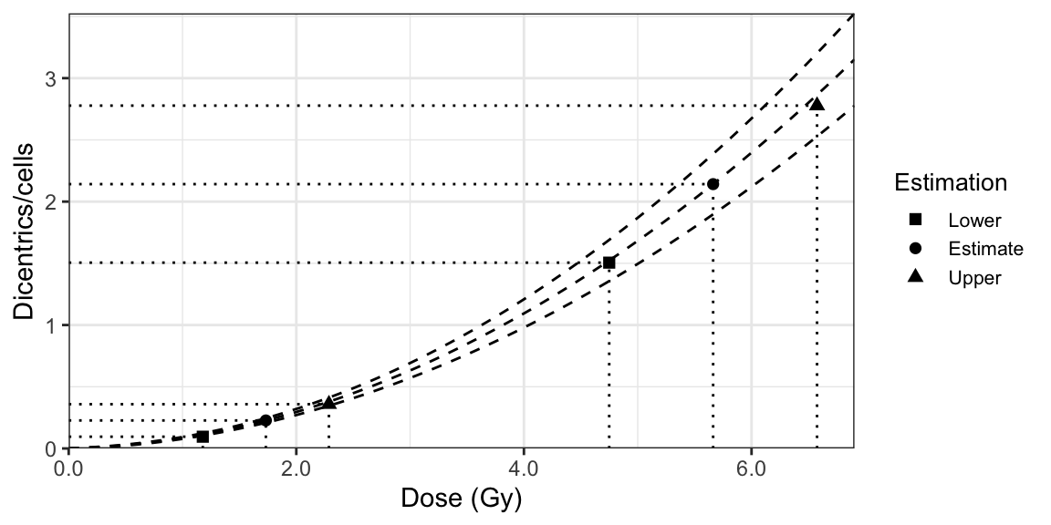
Figure 9.4: A dose-effect calibration curve used to estimate dose uncertainties using heterogeneous method.