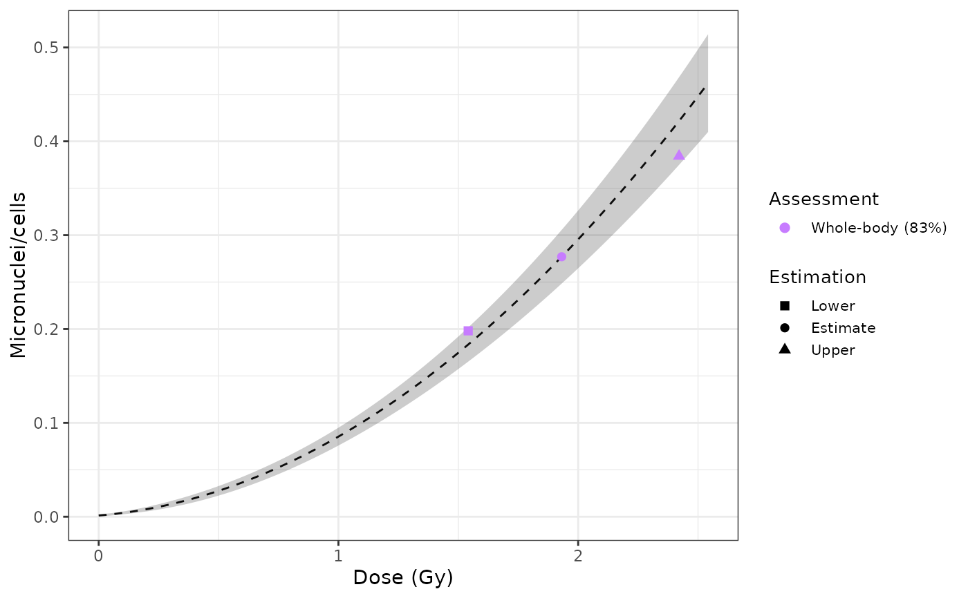
Plot dose estimation curve

Usage

plot_estimated_dose_curve(
  est_doses,
  fit_coeffs,
  fit_var_cov_mat,
  protracted_g_value = 1,
  conf_int_curve,
  aberr_name,
  place
)

Arguments

est_doses: List of dose estimations results from estimate_*() family of functions.
fit_coeffs: Fitting coefficients matrix.
fit_var_cov_mat: Fitting variance-covariance matrix.
protracted_g_value: Protracted \(G(x)\) value.
conf_int_curve: Confidence interval of the curve.
aberr_name: Name of the aberration to use in the y-axis.
place: UI or save.

Value

ggplot2 object.

Examples

#The fitting RDS result from the fitting module is needed. Alternatively, manual data
#frames that match the structure of the RDS can be used:
fit_coeffs <- data.frame(
  estimate   = c(0.001280319, 0.021038724, 0.063032534),
  std.error  = c(0.0004714055, 0.0051576170, 0.0040073856),
  statistic  = c(2.715961, 4.079156, 15.729091),
  p.value    = c(6.608367e-03, 4.519949e-05, 9.557291e-56),
  row.names =  c("coeff_C", "coeff_alpha", "coeff_beta")
)

fit_var_cov_mat <- data.frame(
  coeff_C      = c(2.222231e-07, -9.949044e-07,  4.379944e-07),
  coeff_alpha  = c(-9.949044e-07, 2.660101e-05, -1.510494e-05),
  coeff_beta   = c(4.379944e-07, -1.510494e-05, 1.605914e-05),
  row.names =  c("coeff_C", "coeff_alpha", "coeff_beta")
)

results_whole_merkle <- list(
  list(
    est_doses = data.frame(
      lower = 1.541315,
      estimate = 1.931213,
      upper = 2.420912
    ),
    est_yield = data.frame(
      lower = 0.1980553,
      estimate = 0.277,
      upper = 0.3841655
    ),
    AIC = 7.057229,
    conf_int = c(yield_curve = 0.83)
  )
)


#FUNCTION PLOT_ESTIMATED_DOSE_CURVE
plot_estimated_dose_curve(
  est_doses = list(whole = results_whole_merkle),
  fit_coeffs = as.matrix(fit_coeffs),
  fit_var_cov_mat = as.matrix(fit_var_cov_mat),
  protracted_g_value = 1,
  conf_int_curve = 0.95,
  aberr_name = "Micronuclei",
  place = "UI"
)