Plot fit dose curve

Plot fit dose curve

Usage

plot_fit_dose_curve(fit_results_list, aberr_name, place)

Arguments

fit_results_list

List of fit results.

aberr_name

Name of the aberration to use in the y-axis.

place

Where the plot will be displayed.

Value

ggplot2 object.

Examples

#In order to plot the fitted curve we need the output of the fit() function:
count_data <- data.frame(
  D = c(0, 0.1, 0.25, 0.5, 0.75, 1, 1.5, 2, 3, 4, 5),
  N = c(5000, 5002, 2008, 2002, 1832, 1168, 562, 333, 193, 103, 59),
  X = c(8, 14, 22, 55, 100, 109, 100, 103, 108, 103, 107),
  C0 = c(4992, 4988, 1987, 1947, 1736, 1064, 474, 251, 104, 35, 11),
  C1 = c(8, 14, 20, 55, 92, 99, 76, 63, 72, 41, 19),
  C2 = c(0, 0, 1, 0, 4, 5, 12, 17, 15, 21, 11),
  C3 = c(0, 0, 0, 0, 0, 0, 0, 2, 2, 4, 9),
  C4 = c(0, 0, 0, 0, 0, 0, 0, 0, 0, 2, 6),
  C5 = c(0, 0, 0, 0, 0, 0, 0, 0, 0, 0, 3),
  mean = c(0.0016, 0.0028, 0.0110, 0.0275, 0.0546, 0.0933, 0.178, 0.309, 0.560, 1, 1.81),
  var = c(0.00160, 0.00279, 0.0118, 0.0267, 0.0560, 0.0933, 0.189, 0.353, 0.466, 0.882, 2.09),
  DI = c(0.999, 0.997, 1.08, 0.973, 1.03, 0.999, 1.06, 1.14, 0.834, 0.882, 1.15),
  u = c(-0.0748, -0.135, 2.61, -0.861, 0.790, -0.0176, 1.08, 1.82, -1.64, -0.844, 0.811)
)


fit_results <- fit(count_data = count_data,
                   model_formula = "lin-quad",
                   model_family = "automatic",
                   fit_link = "identity",
                   aberr_module = "dicentrics",
                   algorithm = "maxlik")

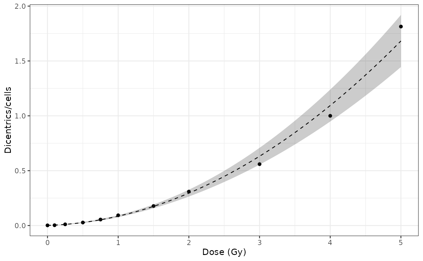
#FUNTION PLOT_FIT_DOSE_CURVE()
plot_fit_dose_curve(
  fit_results,
  aberr_name = "Dicentrics",
  place = "UI"
)