Micronuclei dose-effect fitting

Input count data

The first step is to input the count data. On the {shiny} app, we can select to either load the count data from a file (supported formats are .csv, .dat, and .txt) or to input the data manually. Once the table is generated and filled, the “Calculate parameters” button will calculate the total number of cells ($N$), total number of aberrations ($X$), as well as mean ($\bar{y}$), variance ($\sigma^{2}$), dispersion index ($\sigma^{2}/\bar{y}$), and $u$-value.

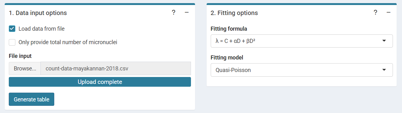
‘Data input options’ and ‘Fitting options’ boxes in the dose-effect fitting module

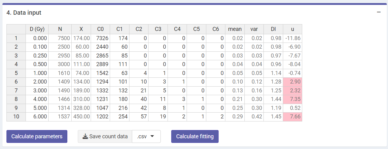
‘Data input’ box in the dose-effect fitting module

This step is accomplished in R by calling the calculate_aberr_table() function:

count_data <- system.file("extdata", "count-data-mayakannan-2018.csv", package = "biodosetools") %>%
  utils::read.csv() %>%
  calculate_aberr_table(type = "count", assessment_u = 1.17)

count_data
#> # A tibble: 10 × 14
#>        D     N     X    C0    C1    C2    C3    C4    C5    C6   mean    var
#>    <dbl> <int> <dbl> <int> <int> <int> <int> <int> <int> <int>  <dbl>  <dbl>
#>  1  0     7500   174  7326   174     0     0     0     0     0 0.0232 0.0227
#>  2  0.1   2500    60  2440    60     0     0     0     0     0 0.024  0.0234
#>  3  0.25  2950    85  2865    85     0     0     0     0     0 0.0288 0.0280
#>  4  0.5   3000   111  2889   111     0     0     0     0     0 0.037  0.0356
#>  5  1     1610    74  1542    63     4     1     0     0     0 0.0460 0.0526
#>  6  2     1409   134  1294   101    10     3     1     0     0 0.0951 0.122 
#>  7  3     1490   189  1332   132    21     5     0     0     0 0.127  0.159 
#>  8  4     1466   310  1231   180    40    11     3     1     0 0.211  0.305 
#>  9  5     1314   328  1047   216    42     8     1     0     0 0.250  0.297 
#> 10  6     1537   450  1202   254    57    19     2     1     2 0.293  0.423 
#> # ℹ 2 more variables: DI <dbl>, u <dbl>

Irradiation conditions

Because irradiation conditions during calibration may influence future dose estimates, and for a better traceability, the user can input the conditions under which the samples used to construct the curve were irradiated. This option is only available in the Shiny app, so that these can be saved into the generated reports.

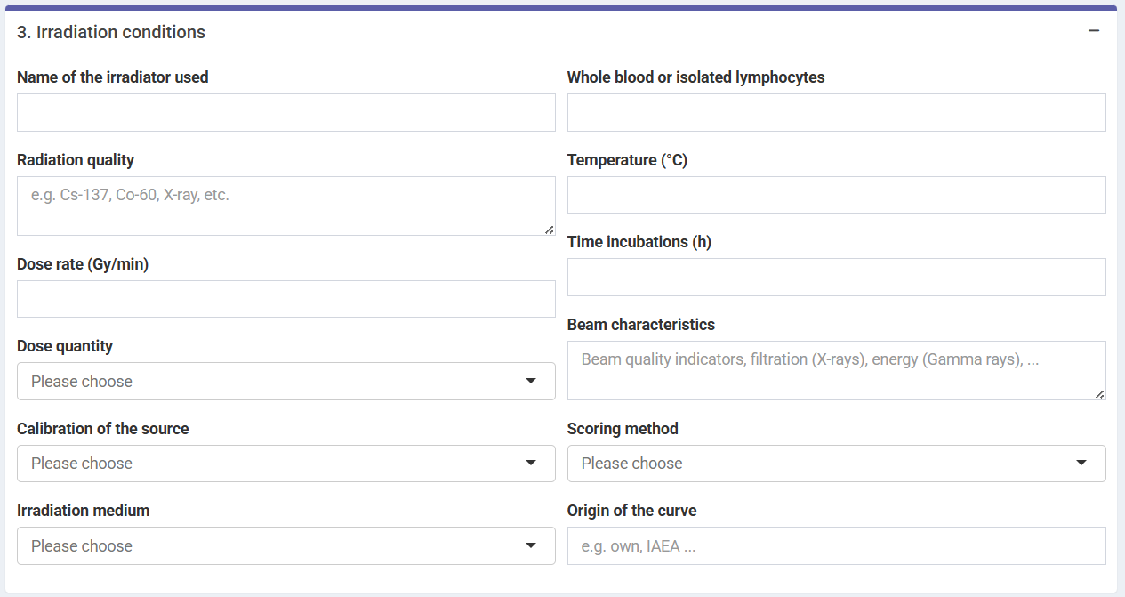
‘Irradiation conditions’ box in the dose-effect fitting module

Perform fitting

To perform the fitting the user needs to select the appropriate fitting options to click the “Calculate fitting” button on the “Data input” box.

The fitting results and summary statistics are shown in the “Results” tabbed box, and the dose-effect curve is displayed in the “Curve plot” box.

The “Export results” box shows two buttons: (a) “Save fitting data”, and (b) “Download report”. The “Save fitting data” will generate an .rds file that contains all information about the count data, irradiation conditions, and options selected when performing the fitting. This file can be then loaded in the dose estimation module to load the dose-effect curve coefficients.

Similarly, the “Download report” will generate a .pdf or a .docx report containing all inputs and fitting results.

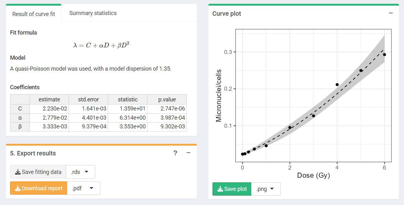
‘Results’ tabbed box, ‘Curve plot’ and ‘Export results’ boxes in the dose-effect fitting module

To perform the fitting in R we call the fit() function:

fit_results <- fit(
  count_data = count_data,
  model_formula = "lin-quad",
  model_family = "quasipoisson",
  fit_link = "identity",
  aberr_module = "micronuclei"
)

The fit_results object is a list that contains all necessary information about the count data as well as options selected when performing the fitting. This is a vital step to ensure traceability and reproducibility. Below we can see its elements:

names(fit_results)
#>  [1] "fit_raw_data"         "fit_formula_raw"      "fit_formula_tex"     
#>  [4] "fit_coeffs"           "fit_cor_mat"          "fit_var_cov_mat"     
#>  [7] "fit_dispersion"       "fit_model_statistics" "fit_algorithm"       
#> [10] "fit_model_summary"

In particular, we can see how fit_coeffs matches the results obtained in the UI:

fit_results$fit_coeffs
#>                estimate    std.error statistic      p.value
#> coeff_C     0.022304968 0.0016412463 13.590263 2.747258e-06
#> coeff_alpha 0.027791344 0.0044014447  6.314141 3.987058e-04
#> coeff_beta  0.003332782 0.0009379284  3.553343 9.301982e-03

To visualize the dose-effect curve, we call the plot_fit_dose_curve() function:

plot_fit_dose_curve(
  fit_results,
  aberr_name = "Micronuclei",
  place = "UI"
)

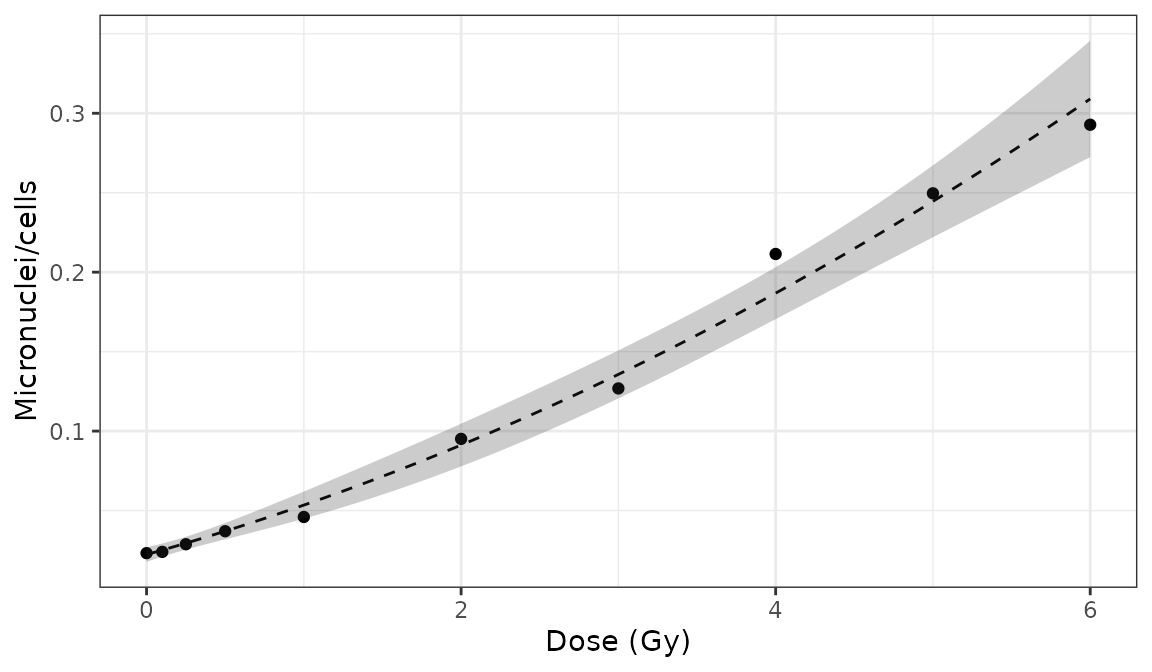
Plot of dose-effect curve generated by {biodosetools}. The grey shading indicates the uncertainties associated with the calibration curve.