Dicentrics dose estimation criticality accidents

Load pre-calculated curves

The first step is to either load the pre-calculated curves in .rds format obtained in the dose-effect fitting module: one for gamma rays and another for neutrons; or input the curves coefficients manually in case the user wants to use a pre-existing curve calculated outside of Biodose Tools.

‘Curve fitting data options’ and ‘.rds input curves’ tabbed box in the dose estimation module for criticality accidents when loading curve from an .rds file.

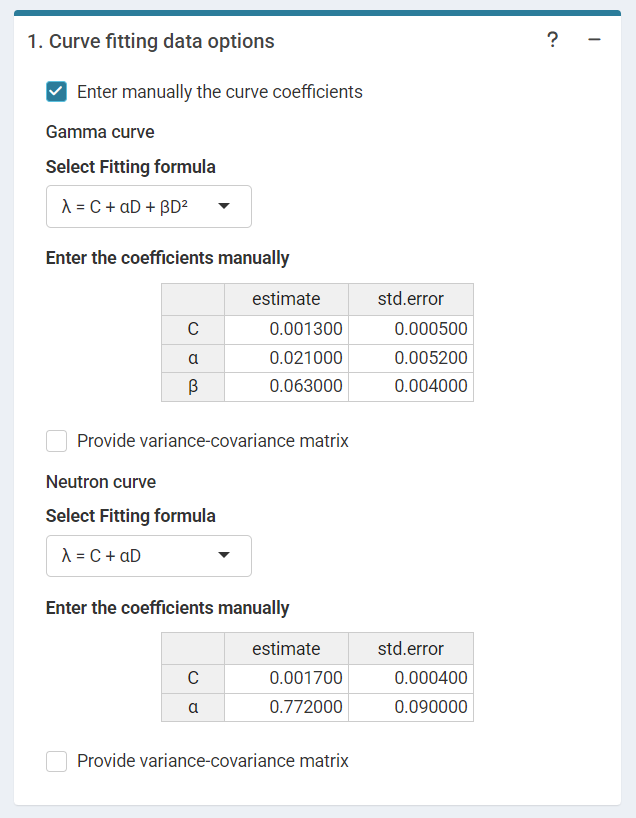
‘Curve fitting data options’ in the dose estimation module for criticality accidents when inputting curve coefficients manually. Note that if no variance-covariance matrix is provided, only the variances calculated from the coefficients’ standard errors will be used in calculations.

This step is accomplished in R by either using load_rds_data() or via load_manual_data():

fit_results_gamma <- system.file("extdata", "gamma_dicentrics-fitting-results.rds", package = "biodosetools") %>%
  readRDS()

fit_results_neutrons <- system.file("extdata", "neutrons-mixed-dicentrics-fitting-results.rds", package = "biodosetools") %>%
  readRDS()

fit_results_gamma$fit_coeffs
#>                estimate    std.error statistic      p.value
#> coeff_C     0.001280319 0.0004714055  2.715961 6.608367e-03
#> coeff_alpha 0.021038724 0.0051576170  4.079156 4.519949e-05
#> coeff_beta  0.063032534 0.0040073856 15.729091 9.557291e-56

fit_results_neutrons$fit_coeffs
#>               estimate    std.error statistic    p.value
#> coeff_C     0.00166593 0.0004100245  4.063003 0.05376763
#> coeff_alpha 0.77187898 0.0899694092  8.579349 0.00665724

Input case data

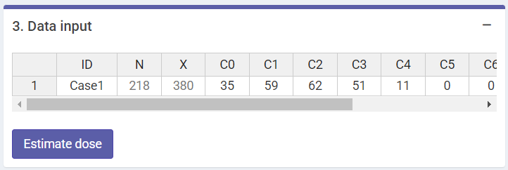
Next we can write a case description in the corresponding box. Then, some parameters must be reported in order to perform the calculations: “Ratio (gamma/neutron)”, “Maximum number of dics per cell”, “Number of cases” and the dicentric distribution (3.Data input). The dicentric distribution table will automatically provide with total number of cells ($N$), total number of aberrations ($X$), as well as mean ($\bar{y}$), standard error ($\sigma$), dispersion index ($\sigma^{2}/\bar{y}$), and $u$-value. An ID column will also appear to identify each case. Multiple cases are supported. Finally, the “Estimate dose” button will give the results.

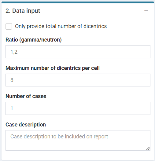
‘Data input’ box in the dose estimation module for criticality accidents.

‘Data input’ box in the dose estimation module for criticality accidents.

Perform dose estimation

Results will appear in green “Results tabs”.

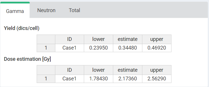
‘Results’ tabbed box, ‘Curve plot’ and ‘Save results’ boxes in the dose estimation module for criticality accidents.

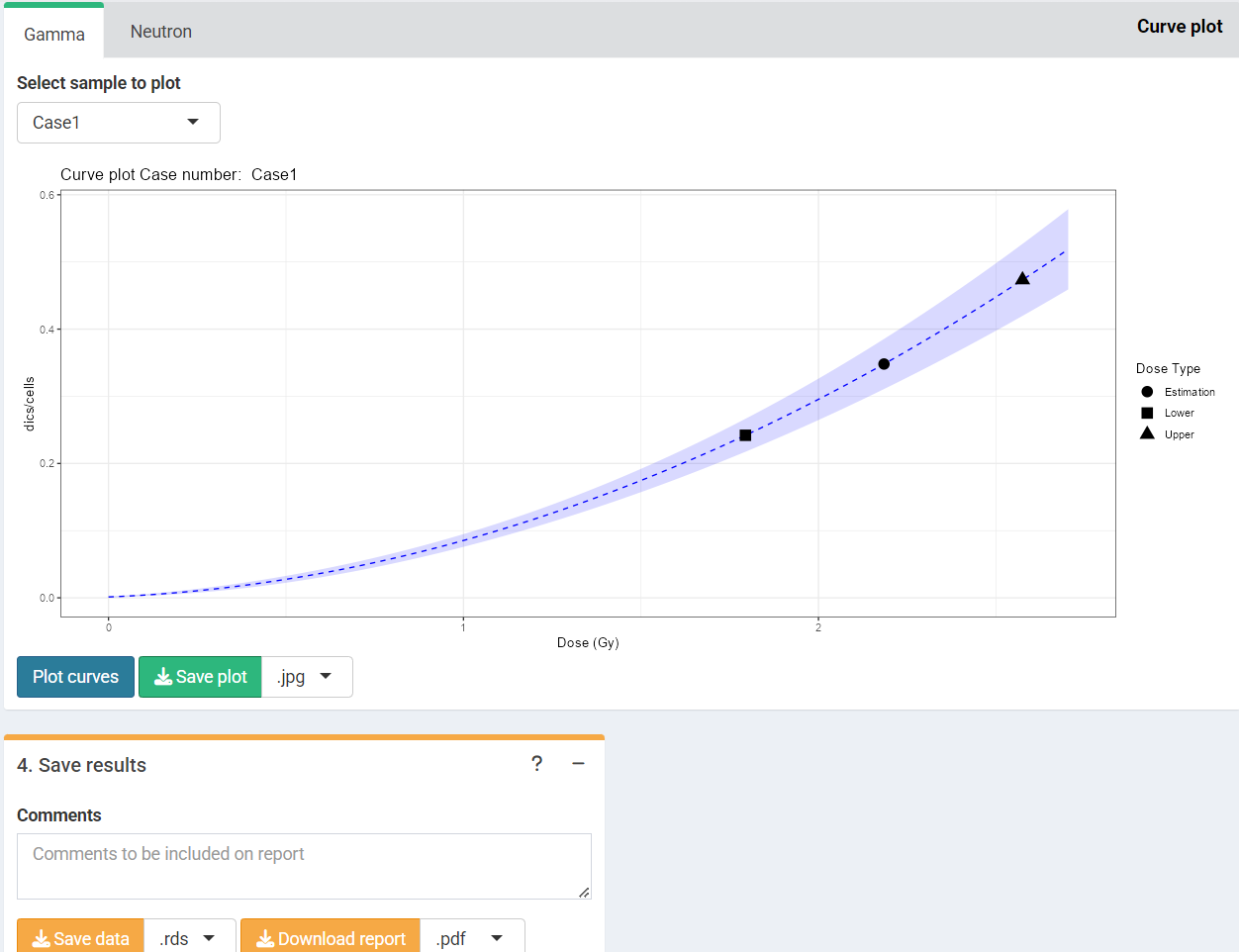
‘Results’ tabbed box, ‘Curve plot’ and ‘Save results’ boxes in the dose estimation module for criticality accidents.

To perform the dose estimation in R we can call fun.estimate.criticality(). First of all, however, we will need to load the fit coefficients and variance-covariance matrix:

coef_gamma <- fit_results_gamma[["fit_coeffs"]][,1]
cov_gamma <- fit_results_gamma[["fit_var_cov_mat"]]
coef_neutron <- fit_results_neutrons[["fit_coeffs"]][,1]
cov_neutron <-  fit_results_neutrons[["fit_var_cov_mat"]]

After that is done, we can simply call fun.estimate.criticality():

est_doses <- fun.estimate.criticality(
  num_cases = 1,
  dics = 380, 
  cells = 218, 
  coef_gamma, 
  cov_gamma, 
  coef_neutron, 
  cov_neutron, 
  ratio = 1.2, 
  p = 0)

est_doses
#> [[1]]
#> [[1]]$gamma
#>      est      lwr      upr 
#> 2.173586 1.784314 2.562857 
#> 
#> [[1]]$neutron
#>      est      lwr      upr 
#> 1.811322 1.486929 2.135715 
#> 
#> [[1]]$total
#>      est      lwr      upr 
#> 3.984907 3.271243 4.698572

To visualise the estimated doses, we call the plot_estimated_dose_curve_mx() function:

plot_estimated_dose_curve_mx(
  name = "Sample1", 
  est_doses = est_doses[[1]], 
  fit_coeffs = coef_gamma, 
  fit_var_cov_mat = cov_gamma,
  curve_type = "gamma",
  protracted_g_value = 1,
  conf_int_curve = 0.95, 
  place = "UI")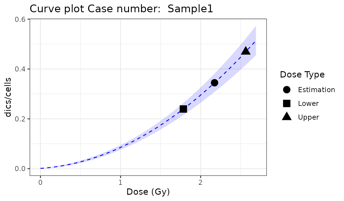

Plot of estimated doses generated by {biodosetools criticality accidents module}. The grey shading indicates the uncertainties associated with the calibration curve.

  

plot_estimated_dose_curve_mx(
  name = "Sample1", 
  est_doses = est_doses[[1]], 
  fit_coeffs = coef_neutron, 
  fit_var_cov_mat = cov_neutron,
  curve_type = "neutron",
  protracted_g_value = 1,
  conf_int_curve = 0.95, 
  place = "UI")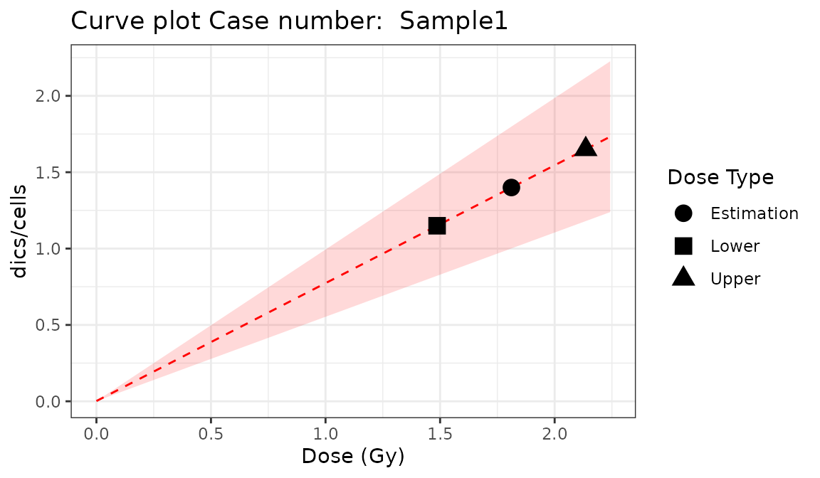

Plot of estimated doses generated by {biodosetools criticality accidents module}. The grey shading indicates the uncertainties associated with the calibration curve.