Dicentrics characteristic limits

Compare proband vs. control

The first step is to input the number of dicentrics and the number of cells counted for the proband (case) and for the control. A significant P-value suggests that the proband was exposed two a dose ($D>0Gy$) and the calculation of the dose shall be performed if an appropriate calibration curve is available.

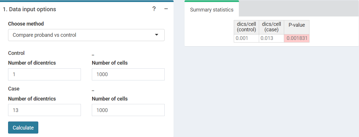
‘Data input options’ in the characteristic limits module - Compare proband vs control method.

This step is accomplished in R by poisson.test() function:

control_data <- c(aberr = 1,
                  cells = 1000)

proband_data <- c(aberr = 13,
                  cells = 1000)
        

result_data <- matrix(c(
    control_data["aberr"] / control_data["cells"],
    proband_data["aberr"] / proband_data["cells"],
    stats::poisson.test(c(proband_data["aberr"], control_data["aberr"]),
                        c(proband_data["cells"], control_data["cells"]))$p.value
      ), ncol = 3, nrow = 1)
    
    colnames(result_data) <- c("dics/cell (control)", "dics/cell (case)", "P-value")

result_data
#>      dics/cell (control) dics/cell (case)     P-value
#> [1,]               0.001            0.013 0.001831055

Characteristic limits

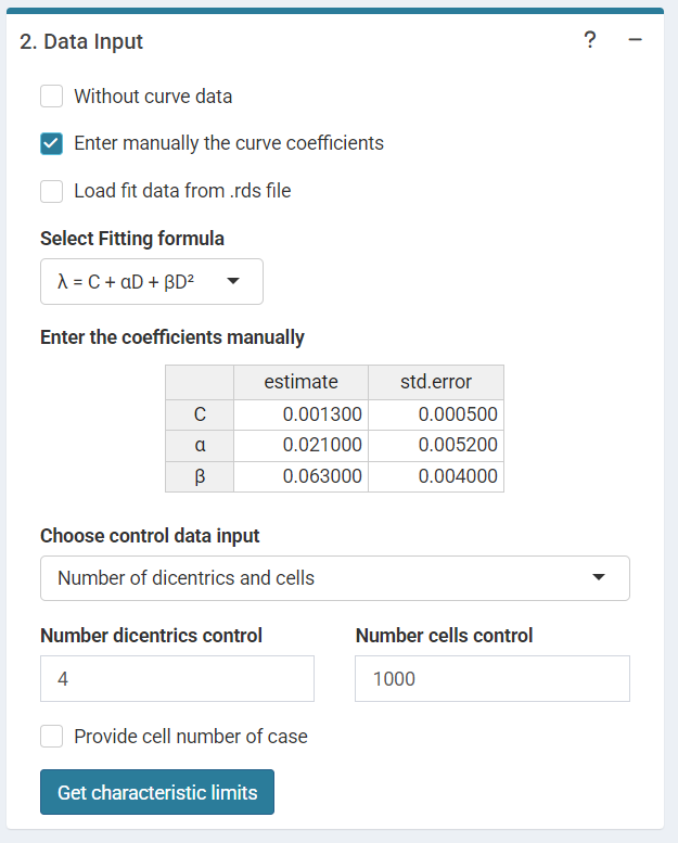
The user can choose the type I error rate($α$)(false positive rate) and the type II error rate ($β$) (false negative rate).

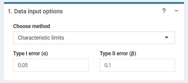
‘Data input options’ in the characteristic limits module - Characteristic limits.

The input data are: the number of dicentrics and cells of the control data if ($Number of dics and cells$) is selected or the mean number of dicentrics per cell if ($Dics per cell$) is selected. Input the pre-calculated curve in .rds format obtained in the dose-effect fitting module.

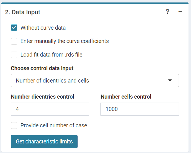
‘Data input options’ in the characteristic limits module - Characteristic limits - Without curve data option.

or input the curve coefficients manually in case the user wants to use a pre-existing curve calculated outside of Biodose Tools.

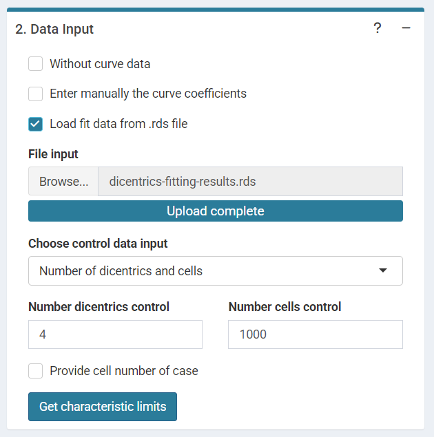
‘Data input options’ in the characteristic limits module - Characteristic limits - Loaded data .rds option.

If these information is not available, choose ($Without curve data$) and the dose will not be calculated.

‘Data input options’ in the characteristic limits module - Characteristic limits - Manually entered curve data option.

This step is accomplished in R by calling the calculate_characteristic_limits() function that gives the decision threshold and the detection limit:

cells_proband <- c(20, 50, 100, 200, 500, 1000)
control_data <- c(aberr = 4,
                  cells = 1000)

c_limits <- sapply(cells_proband, function(x) calculate_characteristic_limits(
  y0 = control_data["aberr"],
  n0 = control_data["cells"],
  n1 = x,
  alpha = 0.05, 
  beta = 0.1, 
  ymax = 100, 
  type = "var"
  ))
  

c_limits
#>                    [,1]    [,2]    [,3]    [,4]     [,5]     [,6]    
#> decision_threshold 1       1       2       3        7        12      
#> detection_limit    3.88972 3.88972 5.32232 6.680783 11.77091 17.78159

For the Minimum resolvable dose ($(Gy)$) and the Dose at detection limit ($(Gy)$) project_yield() function is applied:

fit_results_list <- system.file("extdata", "dicentrics-fitting-results.rds", package = "biodosetools")%>%
  readRDS()
fit_coeffs <- fit_results_list$fit_coeffs[, "estimate"]

 est_dec <- sapply((unlist(c_limits["decision_threshold", ]) + 1) / cells_proband, function(x) project_yield(
   yield = x,
   type = "estimate",
   general_fit_coeffs = fit_coeffs,
   general_fit_var_cov_mat = NULL,
   protracted_g_value = 1,
   conf_int = 0))
  
 est_det <- sapply(unlist(c_limits["detection_limit", ]) / cells_proband, function(x) project_yield(
   yield = x,
   type = "estimate",
   general_fit_coeffs = fit_coeffs,
   general_fit_var_cov_mat = NULL,
   protracted_g_value = 1,
   conf_int = 0))                

est_dec
#> [1] 1.0956559 0.6344613 0.5284423 0.4030546 0.3443595 0.2954731
est_det
#> [1] 1.5918121 0.9474389 0.7560874 0.5662469 0.4503848 0.3712934

Results are displayed in the UI as a table and can be saved in .csv and .tex

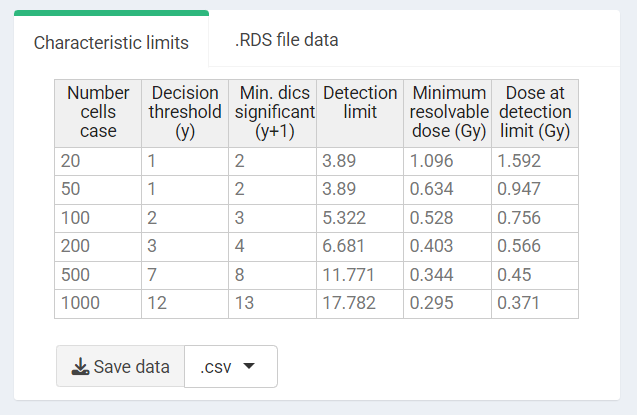
‘Results’ tabbed box in the characteristic limits module - Characteristic limits.